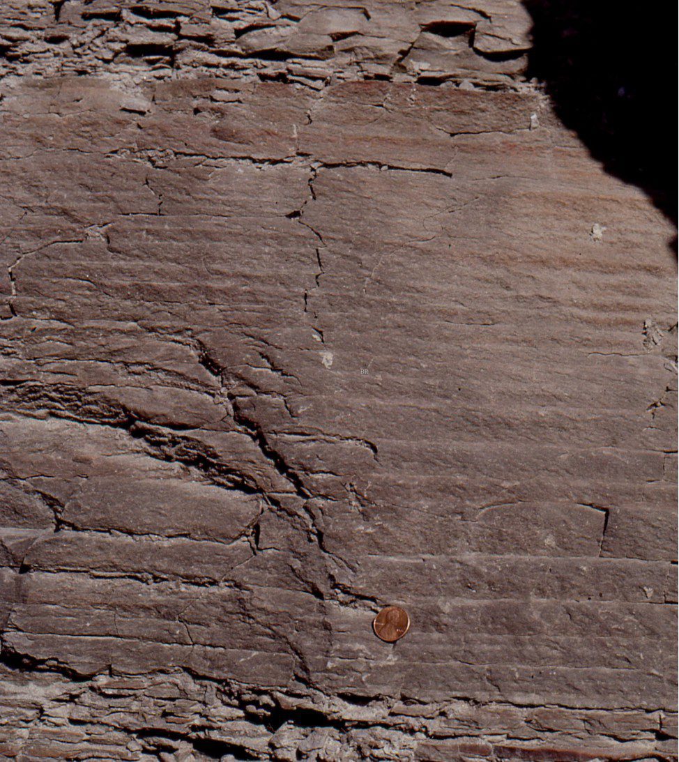
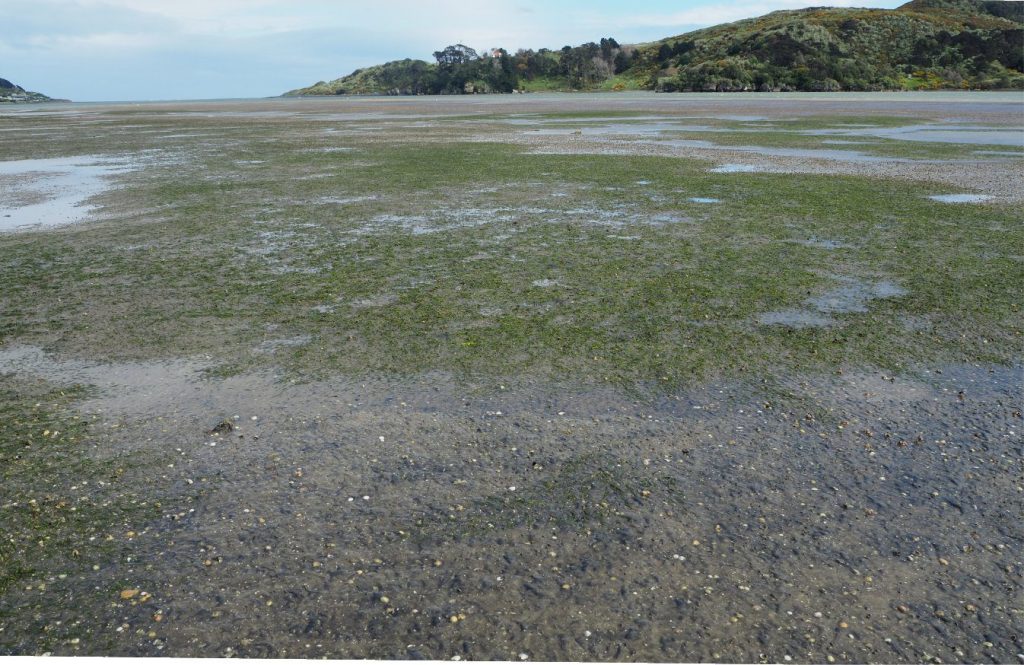
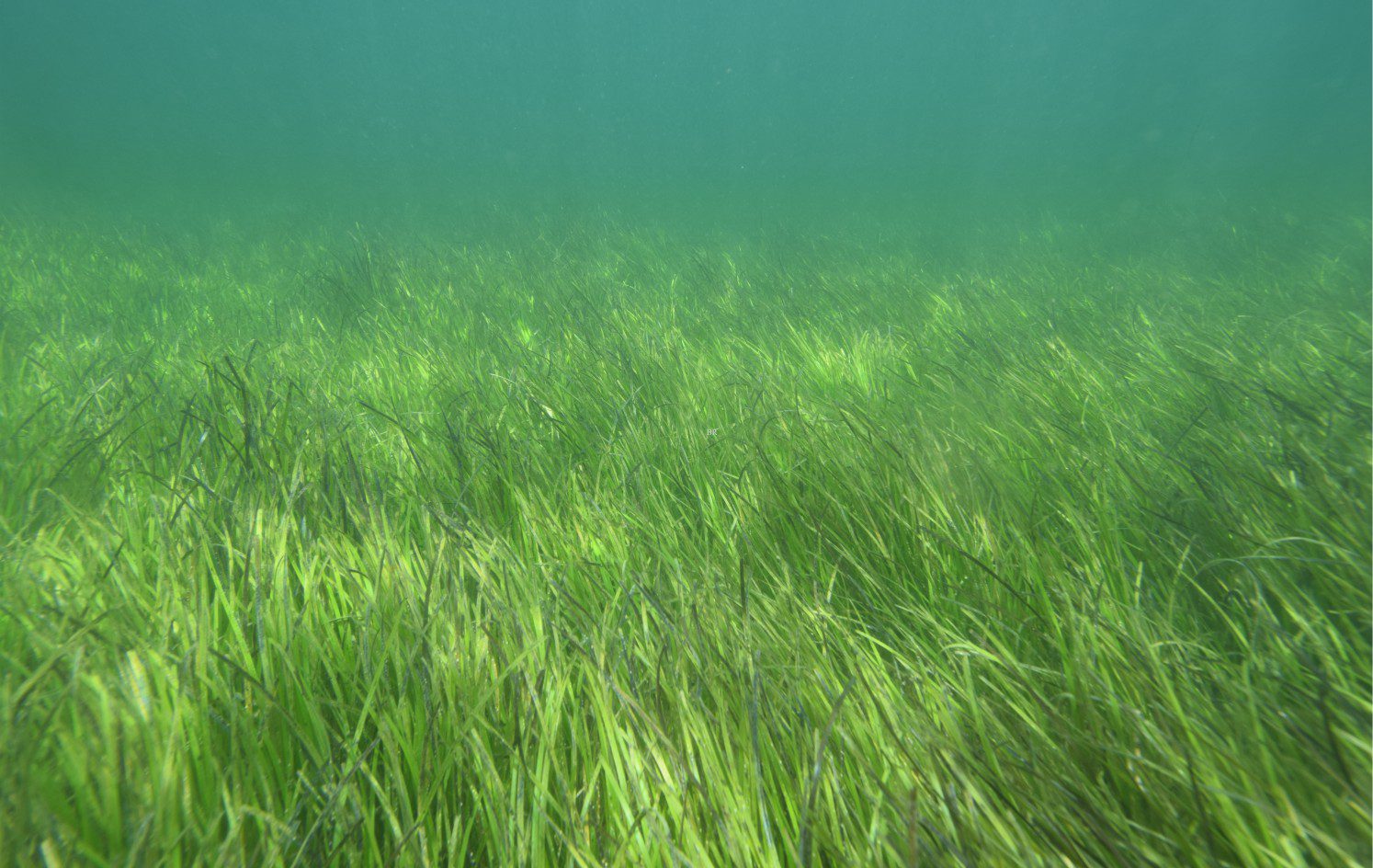
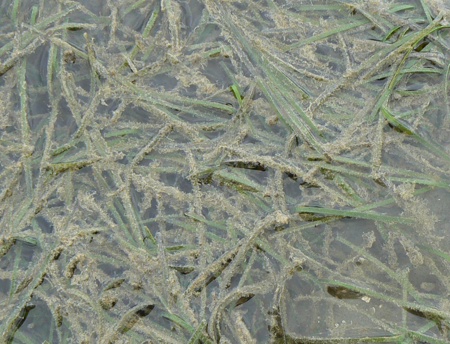
Category Archives: Interpreting ancient environments

Seagrass lithofacies in the rock record

Part of a Zostera marina meadow on sandy tidal flats, Savory Island, British Columbia. Mud content here is <10%. Some leaves are 25-30 cm long. There are a few crustacean or bivalve burrows at left centre.

Some criteria that help us identify fossil seagrasses in the rock record

[This post is a companion to Seagrass meadows and ecosystems]

Coastal seagrasses along with mangrove communities are two of the most productive marine ecosystems in the world. Their primary ecosystem functions have been summarized in a companion post. Despite their importance in modern ecosystems and their presumed contributions to fossil depositional systems, they are poorly represented in the actual rock record. There’s a perfectly logical reason for this – seagrasses are angiosperms, flowering monocotyledons that produce leaves, roots, and rhizomes, all of which are readily biodegradable. Seagrasses have very low preservation potential.

So how is it that seagrass communities are presumed to have been important in Late Cretaceous to Recent coastal paleoenvironments? In a few reported cases there is reasonable direct evidence in the form of leaf-rhizome moulds, casts, and bioimmured fragments. But the main lines of evidence are derived from biofacies associations – the array of epifauna and infauna, motile and sessile invertebrates, protozoa (especially foraminifera), and marine algae (particularly those that secrete calcium carbonate) that indirectly indicate seagrass involvement.

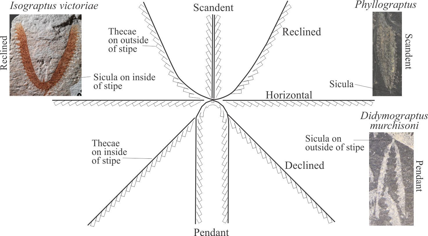
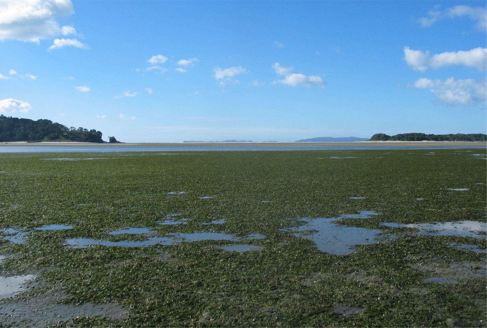
Modern seagrass communities thrive in intertidal and shallow subtidal waters, occurring along most of the world’s coasts from the Arctic-Antarctic circles to the tropics. Species diversity is highest in the tropics. Temperate and cool water coasts have fewer species but those that do exist can develop meadows covering many square kilometres (6 species on the Atlantic and Pacific coasts of Canada; 7 in the Mediterranean, 27 in Australia, and a single species of Zostera along New Zealand coasts). This bioregionalism also means fundamental differences in associated lithofacies and biofacies between tropical and cool-temperate environments.

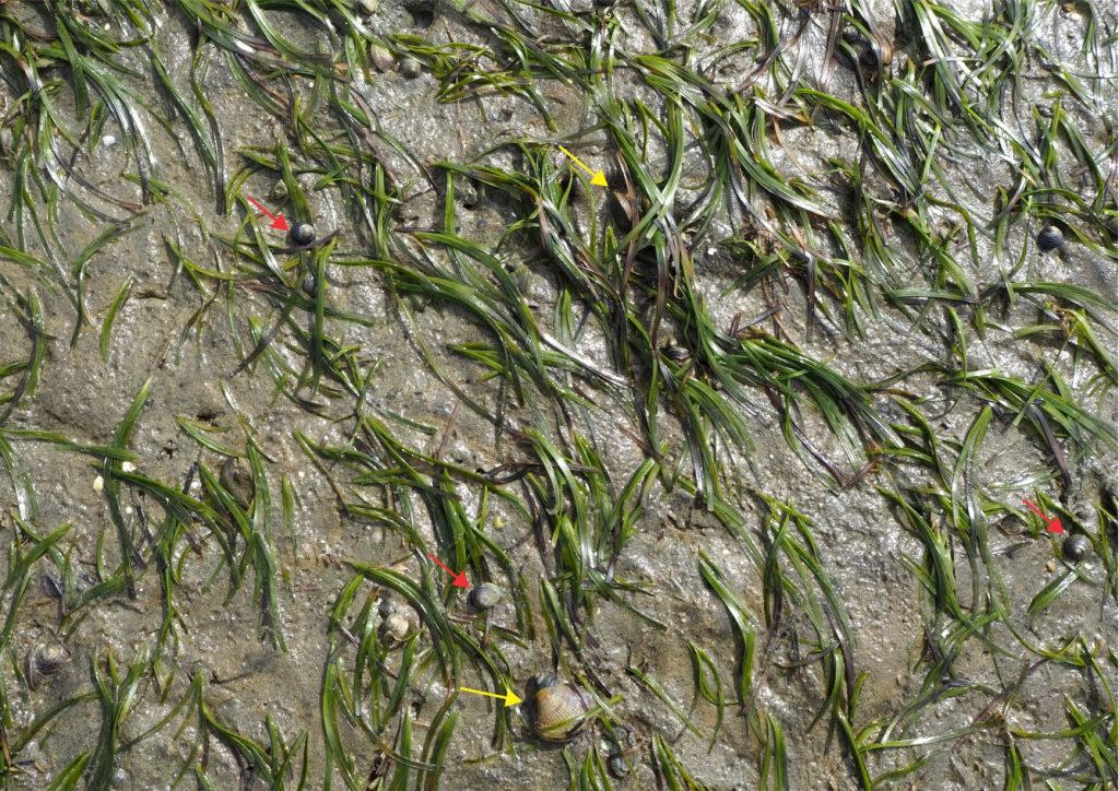
Infaunal activity in this New Zealand example of Zostera muelleri is dominated by (live) buried bivalves (mostly Austrovenus stutchburyi – yellow arrows) and the topshell Zediloma subrostrata (12 specimens in this view – red arrows). There are a few crustacean burrows. The long-spired gastropod Zeacumantus lutulentus is also common (not seen here); both gastropods are scavengers.

In cool and temperate seas, seagrasses are associated predominantly with heterozoan organisms (those that feed on organic matter), phototrophic algae (such as calcareous red algae) and a variety of invertebrates. These associations exist in the modern tropics (with the addition of calcareous green algae), but they share their habitat with or are marginal to coral reefs. Seagrass communities are also regarded as important components of ramp and platform carbonate factories – primarily because of epiphytic organisms such as encrusting foraminifera, bryozoa, and calcareous red algae, and their function as sediment binders and trappers (e.g., Mazarrasa et al., 2015, PDF).

Recognizing ancient seagrass communities

Most publications that identify paleo-seagrass communities do so using indirect criteria; a selection of these papers is linked herein. In a very few cases there is direct evidence where seagrass leaves and rhizomes are preserved intact or as casts, moulds, or impressions. Reich et al., (2015) provide an excellent review of the criteria for seagrass lithofacies recognition, where the evidence is classified as direct (and reliable), or indirect and less reliable (they use terms like “suggestive” and “weak”). Most of the criteria listed by Reich et al., fall into the indirect categories (see their Table 2) – the criteria tend to be weaker because most of the associated invertebrate, protozoa, and algae biofacies are not unique to seagrass communities.

There are some excellent examples of seagrass leaf and rhizome preservation from the Pliocene of Greece and Canary Islands – examples like this are particularly useful for ‘calibrating’ associated fossil biofacies and lithofacies components for application to the more common circumstance where plant fossils are absent.

The examples listed in the table below (certainly not exhaustive) illustrate the range of lithologies and biofacies associations that are used to infer fossil seagrass assemblages.

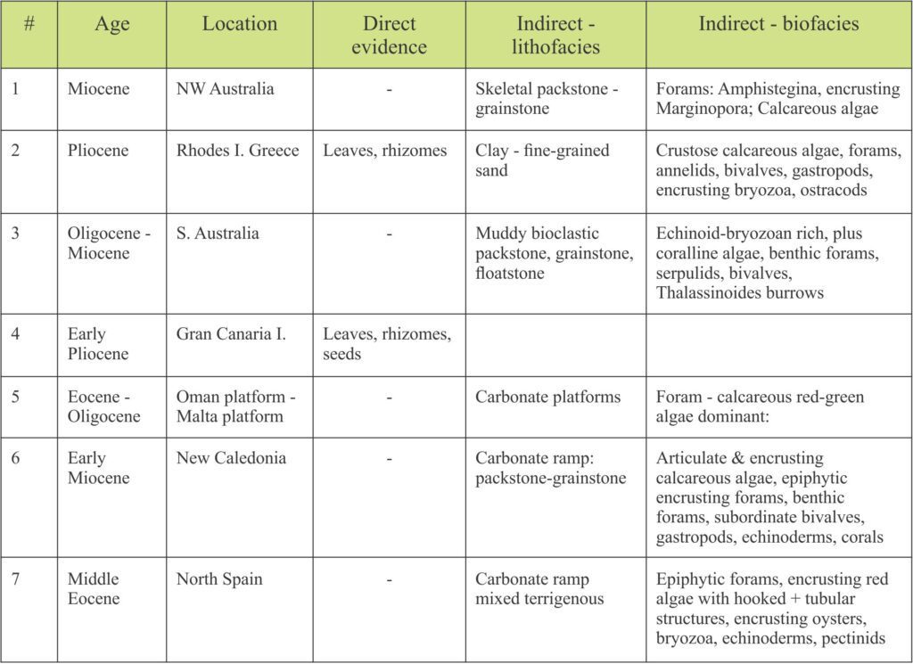
A few examples where direct and indirect criteria have been used to identify fossil seagrass assemblages: 1. Collins et al., 2006, PDF; 2. Moisette et al., 2007. PDF; 3. Riordan et al., 2012; 4. Tuya et al., 2017; 5. Brandano et al., 2019; 6. Elsa et al., 2020, OA; 7. Baceta and Mateu-Vicens, 2022, OA.

Direct evidence

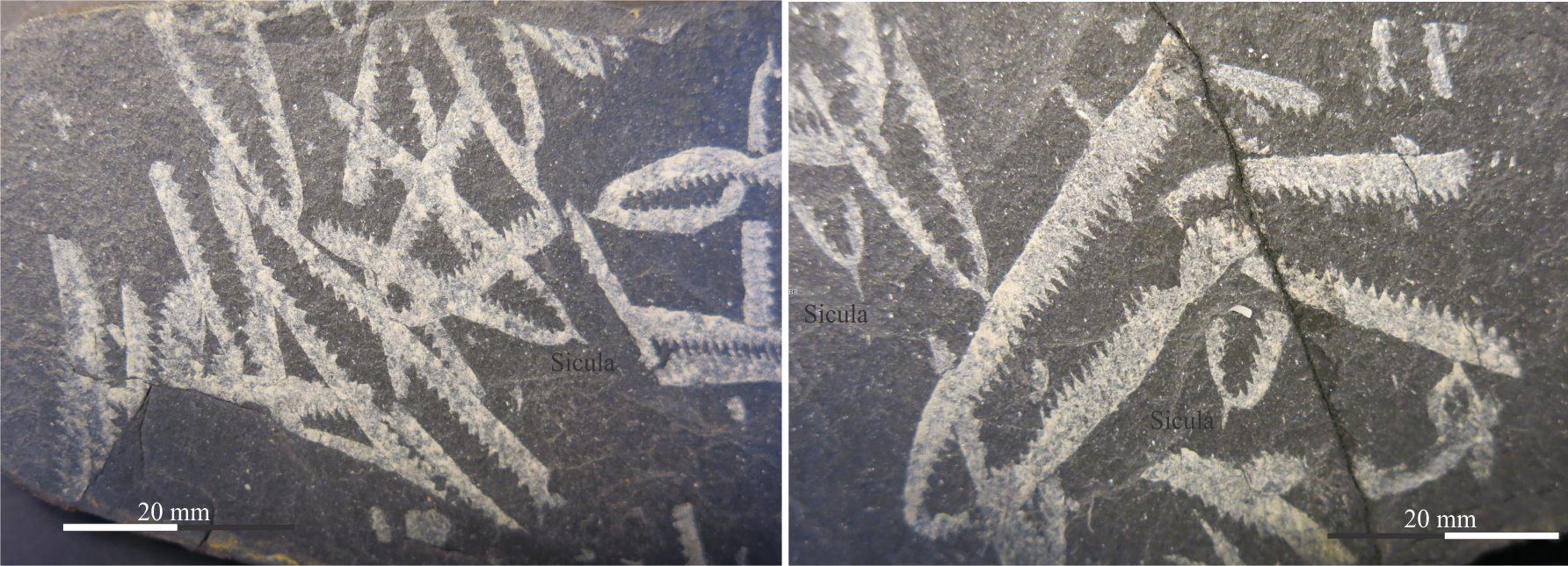
Although rare, seagrass leaves and roots are documented as carbonaceous remains and as impressions in silicified sediment in rocks as old as Campanian. They are also recognizable as bioimmured casts and micritic linings. The degree of confidence with these interpretations is boosted if leaves and stem are attached, and where epifaunal organisms such as bryozoa and calcareous algae are preserved on the leaves. However, it is possible to confuse these fossilized forms with other coastal terrestrial plants or marine macroalgae.

Well preserved fossil leaves and rhizomes have been reported from Pliocene deposits on Canary Islands and Rhodes Island, Greece. The Gran Canaria site also contains seagrass seeds of the species Halodule (Tuya et al., 2017). The Rhodes Island site contains fossil Posidonia oceanica and a rich assemblage of skeletal hydrozoans and invertebrates including crustose coralline algae, foraminifera, annelids, gastropods, bivalves, encrusting bryozoans, and ostracods (Moisette et al., 2007).

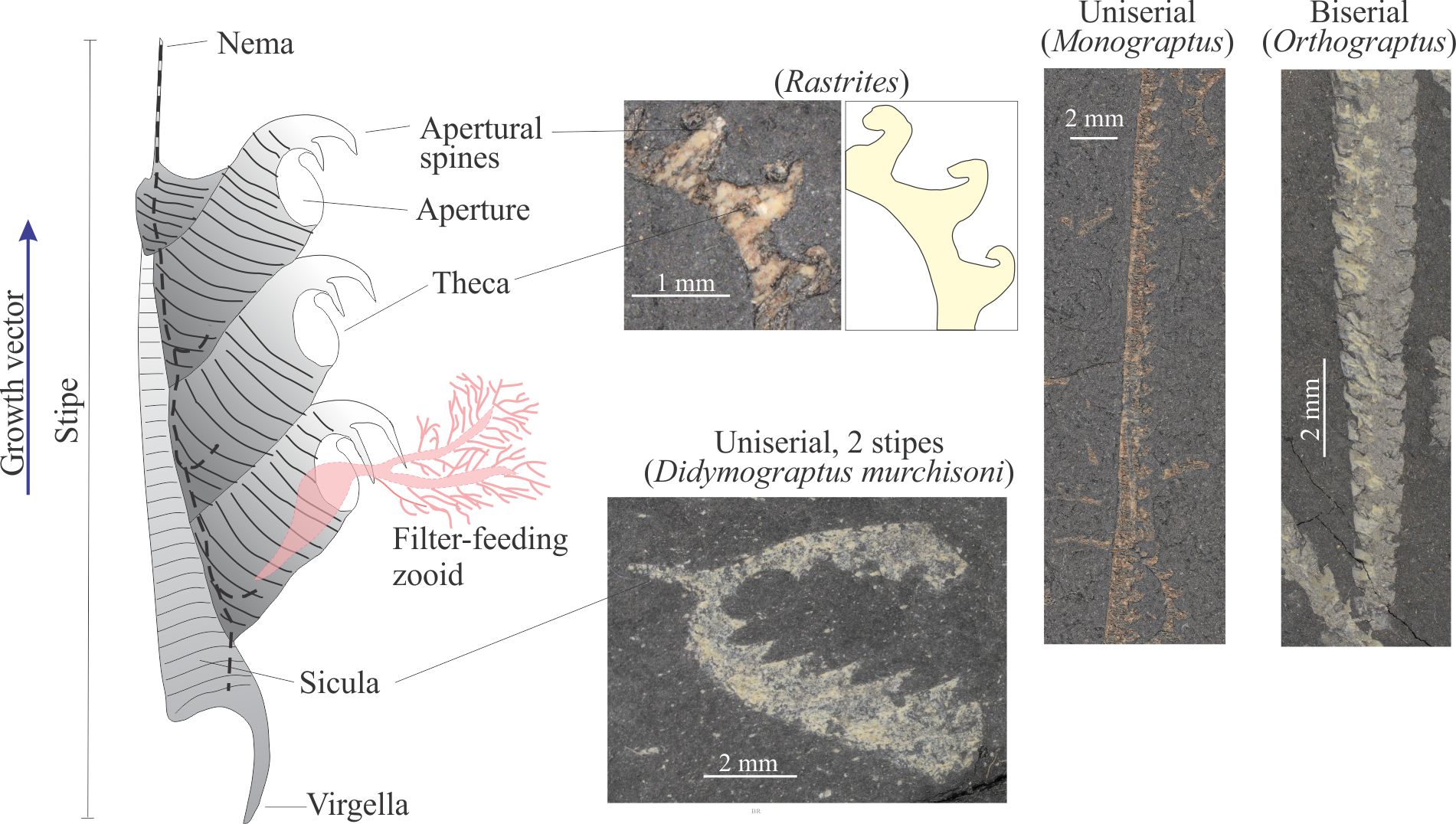
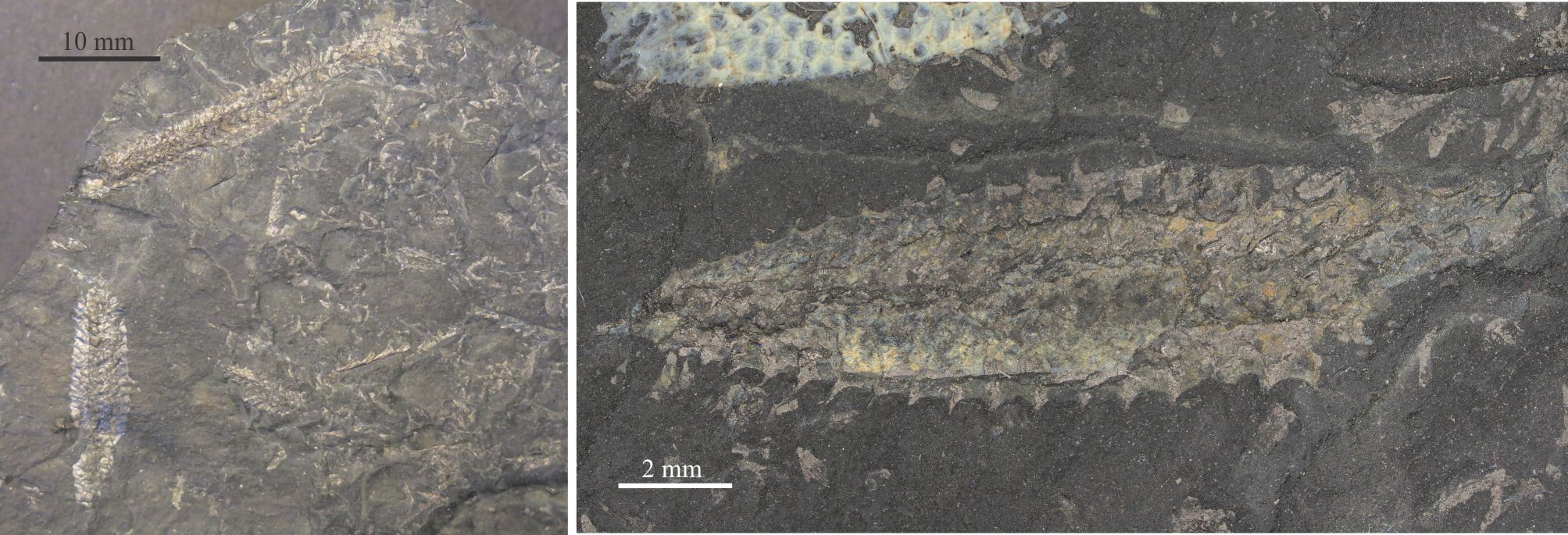
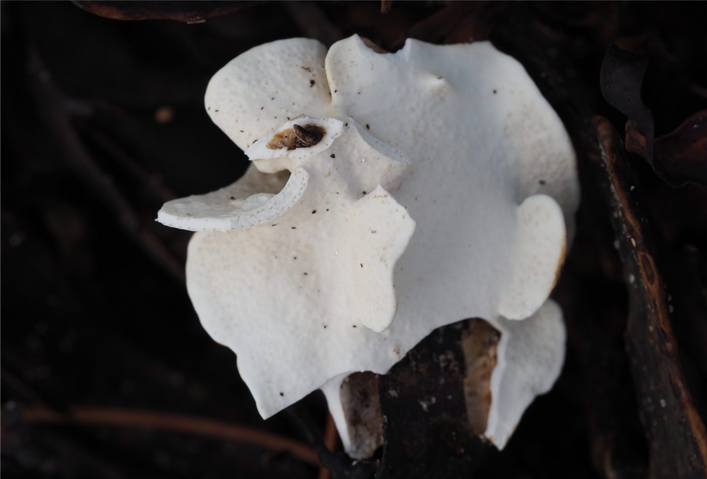
Bioimmuration

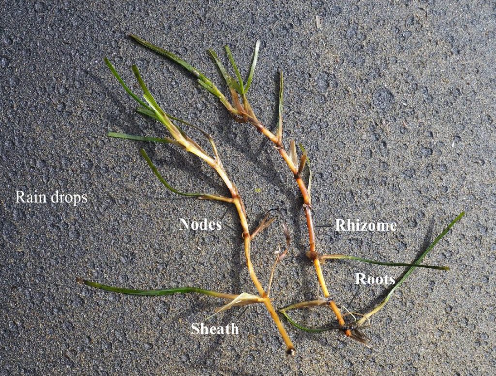
Substratum bioimmuration is the process where the skeletal or encrusting material (commonly calcium carbonate) overgrows another organism. This is particularly important where the substrate is otherwise poorly preserved; for example, plant material or soft-bodied invertebrates. There are a variety of organisms that perform this task – encrusting bivalves such as oysters, bryozoa, crustose calcareous algae, the basal plates of barnacles, and corals. The process has the potential to preserve fine details of the substrate structure – in the case of seagrass, this includes leaf branch nodes, leaf veins, and structures on emergent stems.

Indirect associations

Published interpretations of fossil seagrass communities commonly rely on indirect evidence – the presence (or absence) of associated epifauna on leaves and stems, and infauna that roam, graze, or scavenge the sediment-water interface or dwell within the substrate. Epifaunal and infaunal foraminifera figure prominently in these analyses, commonly in tandem with calcareous algae and bryozoans. Most other invertebrates (e.g., bivalves, gastropods, echinoderms, brachiopods, barnacles, crustaceans) may be important contributors to seagrass ecosystems, but they are not diagnostic as such.

Two structures that improve the confidence with which fossil seagrasses can be identified are:

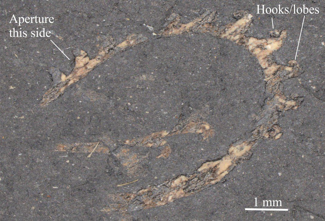
Hook-like structures formed where the encrusting carbonate extends over a leaf edge – they are best observed in thin sections and polished rock slabs, and
Tubular structures where a leaf or stem is completely encased by the encrusting organism. In this case care must be taken to distinguish the encrusting form from superficially similar structures like Serpulid (worm) tubes.

Foraminifera

Motile (can move under their own steam) and sessile forams are common cohabitants with seagrass and in the rock record are the most common group of organisms taken to indicate fossil seagrass communities. This applies particularly to species that are permanently attached to leaves and stems; common examples include the genera Sorites, Planorbulina, and Gypsina . Encrusting species may be preserved attached or bioimurred to seagrass leaf casts. In most cases, preservation potential is high, but a recurring problem is that most attached species also occur on other substrates (e.g., macroalgae, coralline algae), and motile species like Amphistegina and Elphidium are common in other intertidal and subtidal environments.

Calcareous algae

Red algae commonly attach to or encrust seagrass leaves and exposed rhizomes, as they do on other substrates not associated with seagrasses such as brown macroalgae (common seaweeds), mollusc shells, coral rubble, and rock fragments (e.g., Lithothamnion). Crustose species are more likely to preserve seagrass leaves via bioimurration. Hook-like structures formed at leaf crust-overhangs are commonly identified as seagrass leaf artifacts.

Articulate coralline algae (branched, flexible) are more commonly associated with seagrasses than other non-vegetated environments, but even this association is not exclusive. Articulate species are also more likely to detach from the leaf substrate during deposition. Articulate and crustose calcareous red algae are important in both tropical and temperate-cool environments, but may be subordinate to calcareous green algae in tropical settings (e.g., Halimeda, Penicillus).

Calcareous green algae such as Halimeda and Penicillus are photosynthetic, tropical marine dwellers. They are important contributors to carbonate mud factories. They associate with seagrass communities on carbonate platforms and the shallower margins of carbonate ramps, and with a variety of coral reefs in adjacent lagoons or shallow forereef sites.

A forest of articulate calcareous red algae in which there are a few leaves of Zostera muelleri (arrows). The encrusting oyster at left-center is the species Crassostrea glomerata (New Zealand).

Bryozoans

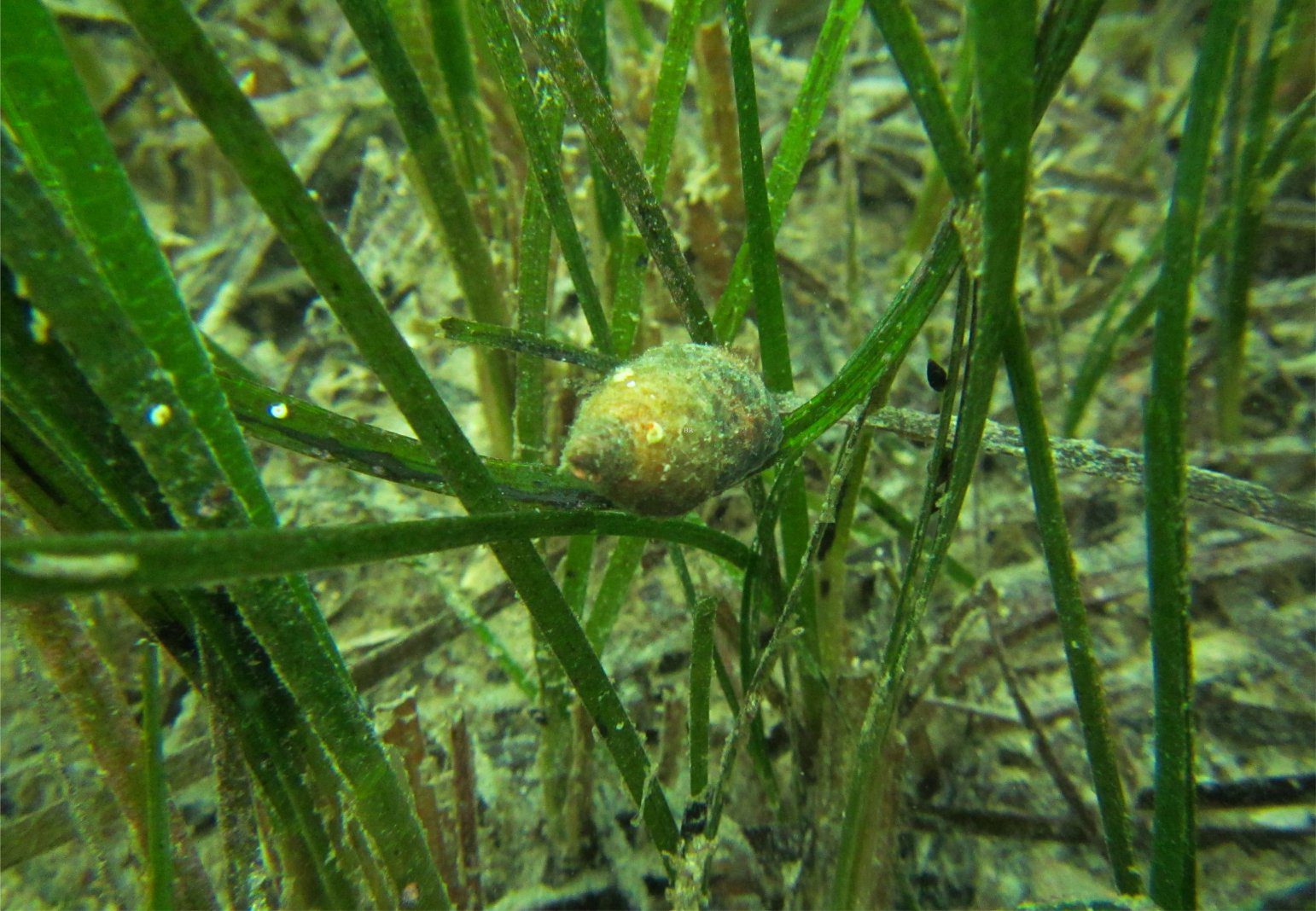
Platey and leaf-like bryozoa can encrust all manner of substrates – in this case a Zostera muelleri rhizome. A remnant of the decaying rhizome is visible at the base of the encrusting mass; the rhizome extended through the circular opening above – the opening is about 3 mm wide.

Bryozoans are a diverse phylum in many shallow marine environments, a diversity that also applies to seagrass communities where both calcareous and non-calcareous species thrive (>150 bryozoa species are associated with some Mediterranean seagrasses; Reich et al, op cit.). Bryozoans that encrust seagrass leaves tend to be unilaminar and less permanent than species that grow on stems and exposed rhizomes – because of leaf flexibility. Colonies that grow on leaves also tend to expand along the length of the leaf and can completely envelop leaves and stems. There may also be evidence for bioimurration of seagrass leaves and rhizomes by encrusting bryozoa (e.g. Taylor and Di Martino, 2014, PDF).

Other invertebrates (bivalves, gastropods, echinoderms)

Infaunal bivalves in many tropical and temperate seagrass communities include the common suspension and deposit feeders (e.g. Venerids, Carditids, Tellinids, and Nuculids), but most of these species also thrive in non-vegetated shallow marine environments. Likewise, epifaunal communities commonly include oysters and Pectinid species, but these too are wide-ranging in other habitats. The mussel family Pinnidae (fan mussels) are common in seagrass substrates but also extend to non-vegetated environments. A similar situation exists for gastropods, although the species Smaragdia may prefer seagrasses. Echinoderms are common inhabitants of seagrass meadows – some species graze on the leaves – but most extend to other non-vegetated settings.

Dense growth of subtidal, upright blades of Zostera muelleri. A gastropod (possibly Cominella adspersa) is grazing epiphytic algae. Bay of Islands, northern New Zealand. Both photos taken by Aleki Taumoepeau, NIWA, Image courtesy of Fleur Matheson, NIWA.

Trace fossils

Given the biological vitality of seagrass communities in intertidal and subtidal environments, it is not surprising that traces and burrows are common in seagrass substrates – we see this in modern depositional settings and their fossil analogues. Burrowing organisms are numerous in these communities – gastropods and echinoderms, crustaceans (crabs, shrimp, sand hoppers); the traces will reflect their diverse behaviours. Common ichnofauna include Thalassinoides, Ophiomorpha, Skolithos, and Scolicia, However, most of these trace fossils are also common in non-vegetated shallow marine settings, so their potential value as seagrass indicators is limited.

Links to the companion posts

Seagrass meadows and ecosystems

Mangrove ecosystems

Mangrove lithofacies

Salt marsh lithofacies

Seagrass meadows and ecosystems

Leave a Reply

Meadows of the seagrass Zostera muelleri exposed at low tide on tidal flats, Raglan Harbour (west coast, New Zealand). They extend into the adjacent subtidal channel. The substrate is fine-grained sand with 10-20% mud. The surface is littered with the shells of the bivalve venerid Austrovenus stutchburyi, a few Macomona liliana (a Tellinid bivalve), and scavenging gastropods. Meadow coverage in this view is a few hundred square metres.

Seagrass meadows are some of the most productive marine ecosystems in the world.

[This is a companion post to Seagrass lithofacies in the rock record]. Four of the images of New Zealand seagrasses were generously donated by Fleur Matheson, NIWA.

I spent much of my childhood wandering the extensive tidal flats and fishing the estuaries of south Waitemata Harbour, the Pacific-fed waterway that embraces east side Auckland, New Zealand. Amongst the many feathered visitors to the tidal flats (between Howick and Beachlands) were huge flocks of black swans that made yearly sojourns to feed on the seagrass meadows. Then, sometime in the late 1960s – early 1970s the seagrass meadows disappeared, along with the swans, the once vibrant and productive ecosystem a victim of widespread pollution and sediment flux across the entire harbour (caused by coastal development, reclamation, storm water runoff, and fertilizer-herbicide runoff). This is a familiar story along many NZ coasts – a microcosm of the global problem of coastal degradation. Coastal seagrasses along with mangrove communities are two of the most productive marine ecosystems in the world – they are also the most threatened.

A Zostera meulleri meadow gracing the intertidal shore of Whangapoua Harbour, northern Coromandel, New Zealand. Image courtesy of Fleur Matheson, NIWA.

Seagrass communities

Like fields of wheat, submerged seagrass meadows sway with the passing waves and tidal currents. Despite this poetic analogy, the word element ‘grass’ is a misnomer. Seagrasses are monocotyledons, the group of terrestrial angiosperms that develop a single embryonic leaf (dicotyledons develop two embryo leaves). Seagrasses evolved a tolerance to saline conditions from their Late Cretaceous terrestrial ancestors. Like their terrestrial cousins, they develop extensive root systems, produce flowers, and are pollinated while submerged by all the critters that graze, hide, or live within their leafy corridors. Seagrasses are not related to seaweed and other forms of algae – macroalgae are attached by holdfasts rather than roots; algae do not produce flowers. Eelgrass and turtle grass are a couple of common names.

A very nice shot of subtidal Zostera muelleri, swaying in unison with each passing wave. Urupukapuka Island, northern New Zealand. Photo taken by Rohan Wells, NIWA, Image courtesy of Fleur Matheson, NIWA.

Seagrasses have relatively limited species diversity (60 or 72 species world-wide depending on who you talk to) but they are widely distributed across temperate and tropical coasts. Temperate varieties grow in estuaries, bays, and lagoons, forming extensive meadows between mangroves or salt marshes, and the seaward continuation of tidal and subtidal flats. Tropical varieties also grow in these settings including shallow lagoons behind coral reefs. They tend to avoid coasts that are subjected to high energy wave conditions (e.g., open seas surf zones) where substrates are continually reworked. And like mangrove communities, they help protect coastal areas from strong tidal currents and storm wave attack.

Water depths

Seagrasses thrive in waters shallow and clear enough to permit sufficient light penetration (for photosynthesis). Meadows that develop on tidal flats are subject to diurnal submergence. Some species also thrive in subtidal settings, usually limited to the shallowest few metres of the photic zone but they have been found as deep as 90 m. Frequent periodic or continuous submergence is a prerequisite for their survival. A few genera such as Posidonia are restricted to subtidal conditions, others extend across the range of water depths (e.g., Zostera, Thalassia). They prefer substrates that are not continually reworked by strong currents and energetic waves, which means they usually avoid open coasts with surf zones. They also avoid areas subjected to desiccation.

Physical characteristics

Rhizomes, leaves, and roots of Zostera muelleri. Leaf stems and roots can develop on the same rhizome nodes. These specimens are 15 cm long; the leaves have been shortened by grazers.

The most common seagrass morphotypes produce long, narrow, flexible leaves with a longitudinal vein. Eel grass and Turtle grass are of this type. Leaves occur singly or in multiples attached to a rhizome via a papery sheaf. Leaf length is variable among species but commonly is 15 cm and more. Leaf margins are smooth. A few smaller species produce more oval-shaped leaves, each attached by a single stem to a rhizome; other small species are compound with multiple leaves arranged in opposite fashion on a single stem (Morrison et al., 2011, PDF).

Rhizomes have a thick, stringy appearance. They are segmented, separated by nodes from which leaf stems and new rhizomes extend. Much finer roots spread from the rhizomes. Rhizomes spread laterally within the substrate – they are only exposed by erosion or predation.

Seagrass substrates

The following characteristics provide context for fossil substrate lithofacies; most of the data is from Piñeiro-Juncal et al., 2022 (PDF available) who review the physical and chemical properties of seagrass soils.

Dense growth of Zostera muelleri on an exposed tidal flat. The long, skinny leaves are aligned parallel to the direction of the outgoing tidal flow. The substrate here is sandy with 10-20% mud. Ripples that abound on the non-vegetated tidal flats are not present across the meadows because the seagrass has dampened wave and current flows. Small trails (bottom right) were made by the gastropod topshell Zediloma subrostrata.

Seagrass substrates can be classified as marine soils: Although they are not always referred thus in the sedimentological literature, the substrates possess many of the characteristics of their terrestrial soil counterparts – they occur at the sediment-water interface and are subjected to physical, chemical, and biological processes, they are granular, contain organic matter, water, micro- and macrobiota, and gasses (in this case dissolved oxygen and carbon dioxide), and provide the foundation for plant life.
Composition: Seagrasses grow in siliciclastic, carbonate, and mixed carbonate-siliciclastic sediment that is unconsolidated. Carbonate substrates of the tropical kind will potentially contain abundant fragmental reef framework coral, calcareous algae (framework species like Lithothamnion, plus green algae mud producers such as Renalcis and Halimeda), and bryozoan fragments, in addition to diverse invertebrate and protozoa shells and tests. Temperate-cool water carbonate substrates are dominated by non-reef forming invertebrates such as molluscs, barnacles, bryozoa, echinoderms, crustose and articulated calcareous algae, and protozoa such as foraminifera. Most seagrass species are adapted to sandy sediments – measured mud volumes are generally less than 25%. Some species tolerate higher mud contents, others prefer <10-15% mud.
Root zone: Long-lived meadows develop a dense tangle of roots and rhizomes that potentially obliterate all primary sedimentary structures. Compared to seagrass leaves, these root masses have relatively high preservation potential, particularly the thicker more robust rhizomes that may be preserved as casts or molds (e.g., by precipitated iron oxides, calcite, aragonite).
Infaunal burrowing: A diverse benthic fauna will include various invertebrates that crawl or burrow into the root-bound substrate. Distinguishing burrows that have distinct linings, branching, or infill structures (e.g., meniscus structures, or Ophiomorpha nodules) from root-rhizome casts or molds should be relatively straight forward. Simple burrows or trails may be more difficult to distinguish.
pH: Average measured soil-water pH values range from 6.9 and 8.2. A few observations indicate that pH is higher in the upper few centimetres of soil/substrate, becoming more acid below where the rhizome concentration is greatest. The presence of carbonate tends to present higher pH values. Measured organic carbon contents average <2-3%, but range to 10% and more.

Seagrass ecosystem functions

Like mangrove communities, seagrasses are critical components of shallow coastal environments from both ecosystem and human perspectives (in a sense they are the same perspectives). The following functional criteria have been gleaned from Duffy, 2006; Matheson et al., 2009; Morrison et al., op cit; Short et al., 2007, PDF.

The high organic matter production that, during photosynthesis absorbs CO₂, becomes part of the biogeochemical equation of seawater pH buffering. The organic matter also serves as part of the food chain both as live ‘forage’ (e.g., turtles, birds, echinoderms), and as particulate and dissolved components that become part of the food web for reefs, hydrodynamic invertebrate buildups (e.g., oysters), and other seafloor communities.
Sediment substrates are stabilized by seagrass root masses and the leaf clusters help attenuate wave energy and tidal currents. An additional outcome of sediment stabilization and trapping is the recycling of nutrients from plant breakdown, nutrients that are important for seagrass growth.

Dense growth of subtidal, upright blades of Zostera muelleri over a litter of dead leaves, the breakdown of a which provides nutrients to the seagrass meadow and soil microbes. Bay of Islands, northern New Zealand. Photo taken by Aleki Taumoepeau, NIWA, Image courtesy of Fleur Matheson, NIWA.

Seagrass leaves provide a template for epifauna and epiflora (e.g., bryozoa, foraminifera, micro-algae) that become a food source for grazing fish and invertebrates such as crustaceans and gastropods.

Dense growth of Zostera muelleri exposed at low tide. The filigree coatings on the leaves are epiphytic algae that are a food source for a variety of grazing invertebrates. Image courtesy of Fleur Matheson, NIWA.

Dense meadows provide shelter for fish, invertebrates, protozoa (e.g., foraminifera) and commonly act as nurseries for fish, crustaceans such as shrimp, and many species of mollusc, including commercially important species. These nurseries provide protection for juvenile fish, and a platform for fish and gastropod eggs. Neighbouring species groups include polychaetes (worms), echinoderms (grazers), bryozoa and sponges.

Infaunal activity in this New Zealand example of Zostera muelleri is dominated by (live) buried bivalves (mostly Austrovenus stutchburyi – yellow arrows) and the topshell Zediloma subrostrata (12 specimens in this view – red arrows). There are a few crustacean burrows. The long-spired gastropod Zeacumantus lutulentus is also common (not seen here); both gastropods are scavengers.

Fish and invertebrate diversity tend to increase in areas where seagrasses thrive (similar to mangrove communities). Invertebrate diversity is also important because many species will graze macro- and microalgae that compete for the same seagrass niche.
Seagrass leaves on tidal flats are foraged by birds and in subtidal environments by sea turtles, dugongs, and manatees.
Seagrass communities are indicators of environmental health – acting as the ‘canary in the cage’ for eutrophication and pollution of waterways, rising seawater temperatures, and competition for their niche by invasive flora and fauna. There is a well-documented example from the 1930s when an invasive mold pathogen all but eliminated seagrass communities along most North Atlantic coasts (Short et al., op cit.). The disappearance of these communities meant that coexisting ecosystem components such as molluscs and shrimp also disappeared or moved to new neighbourhoods. Invasion of seagrass communities by non-native invertebrates from shellfish aquaculture farming has also been recorded on several British Columbia coasts (Mach et al., 2015).

Link to the companion post

Seagrass meadows and ecosystems

Seagrass lithofacies in the rock record

Mangrove ecosystems

Mangrove lithofacies

Salt marsh lithofacies

Graded-bedding lithofacies

Leave a Reply

Controlled experiments on turbidity currents allow us to observe the dynamics of flows and the organization of their deposits. Phillip Kuenen and Carlo Migliorini (1950) conducted experiments like the one shown here – they were able to reproduce the kind of graded bedding observed in many outcrops, setting in motion a scientific rethinking of deep-sea sedimentary processes that still resonates today.
The experimental flow shown above was designed to sample the concentration of sediment suspended in the turbulent plume over the duration of the flow (using siphons). Four time-lapse images show different stages of flow development, with two of the siphons at 8 m and 11.6 m from the flume inlet. The inset curve plots flow velocity with distance along the flow path. Image credit: Modified slightly from O.E. Sequeiros et al., 2009. Figure 5, Experimental study on self-accelerating turbidity currents. J Geophysical Research; Oceans

Historical context

The name graded bedding was coined by E. Bailey in 1930 to describe the gradual, vertical change in grain size within a depositional unit (a bed), from coarse-grained at the base, to fine-grained at the top. To comply with his definition, Bailey insisted that the grain size transition should not be interrupted by crossbedding or erosional surfaces. The term could be applied to almost any grain size transition. Bailey surmised that graded bedding formed when sediment was introduced to the water column from volcanic eruptions, dust storms, and river flood plumes, or initiated by earthquakes – the bigger, heavier lumps would fall from suspension fastest, followed by successive deposition of progressively finer material, or from rivers during the waning stages of floods. His interpretations were perfectly reasonable for some examples of graded bedding, like those found in varves, the deposition of air-fall volcaniclastics in water, and from hypopycnal plumes. However, there was one group of rocks for which the explanations offered by Bailey and his contemporaries fell short – the thick, seemingly monotonous successions of flysch.

Flysch, the German word for flow, was applied in the early 19^th C as a stratigraphic descriptor for thick successions of interbedded shale and sandstone (plus a few subordinate lithologies). It was primarily a European term used to describe rocks associated with the Tertiary Alpine Orogeny. Multi et al., (2009, PDF available) provide a nice summary of the history of its usage. A characteristic feature of flysch sandstone beds is their graded bedding; associated lithofacies and sedimentary structures include scoured basal contacts, and finer grained lithologies containing ripples, climbing ripples, and convoluted laminae. Flysch sandstones also tend to be muddy, where the coarsest grain size fractions are mixed with some of the finest grain sized materials (clay, silt), although the proportion of clay and silt increases upwards in each bed.

A thick, seemingly monotonous (really, it isn’t) Paleoproterozoic flysch-like turbidite succession (stratigraphic top to the left). Most beds are graded, and in Bouma model notation contain varying combinations of A, B, C, D, and E depositional units. In this view, the thicker beds also have graded A, B, or A-B divisions. Variations in bed thickness and the proportions of Bouma divisions probably reflect the changing dynamics of active submarine fan lobes. Belcher Islands, Hudson Bay. Field notebook on lower left.

Graded sandstone beds in flysch are repeated in a seemingly endless progression through stratigraphic successions 100s of metres thick. And this was problematic for pre-1950s geoscientists because it required an explanation that provided a mechanism for events repeated 1000s of times – a mechanism that also explained their textural properties. Invoking flood-generated plumes, storm erosion and suspension of sediment, volcanic eruptions, repeated earthquakes, or rapid tectonic uplift and subsidence of a basin floor (a yo-yo like process), didn’t quite meet the requirements. Any of these mechanisms might explain a few depositional events, but not 1000s of them. Likewise, the bathymetry in which they were deposited was also problematic, particularly with the discovery of sand beds in the deep ocean basins, 100s of kilometres from shore; how on Earth did they get there? Enter Phillip Kuenen and Carlo Migliorini (Kuenen and Migliorini, 1950): This duo combined Kuenen’s expertise in experimental sedimentology and Migliorini’s geological field knowledge (Mutti et al., 2009, op cit).

A Paleocene, flysch-like succession of thin-bedded turbidites and mudstones nicely exposed at Point San Pedro, California (top to the right). This exposure is interesting because there are stratigraphic changes in bed thickness: a laminated and rippled mud-dominated package (left) abruptly overlain by three thinning upward sandstone-shale packages (top to the right). The former may represent deposition on the more distal part of a submarine fan lobe (compared with the thick bedded, Paleoproterozoic turbidites shown above); the latter may be the distal fringes of submarine fan lobes, or interchannel overbank deposits.

Although Kuenen and Migliorini are usually credited with introducing the term turbidity current, the existence of density-driven, bottom-hugging sediment-water flows had been known for some time before 1950 and it seems that D.W. Johnson may have pre-empted them in his book The Origin of Submarine Canyons (1939). Density-driven currents had been observed in Lake Mead (reported by Daly, 1936, Gould, 1954 p. 201-207, and others) where they were described as turbid flows, density currents, or gravity-driven flows, mostly generated from plunging sediment plumes (that we would now call hyperpycnal flows). But it was Kuenen and Migliorini’s 1950 paper detailing the proposition that turbidity currents were responsible for the graded beds found in flysch, that set in motion a complete rethinking of deep-sea sedimentation and deep-water depositional processes – so much so that subsequent recording and interpretation of graded bedding has become intertwined with the concept of turbidites and deposition from subaqueous, turbulent density flows.

The Kuenen-Migliorini experiments yielded two notable (and reproducible) results:

Elucidation of the structure and density of the turbulent flows themselves, particularly the dynamics at the flow head, tail, and overlying plume.
The reproduction of graded bedding that proved almost identical to outcrop versions in overall appearance and grain size distribution.

The grain-size distributions for one of their experimental flows are shown below (redrawn from their Figure 5). The histograms represent samples taken at successive distances above the base of the turbidite flow unit. Two observations of note are:

There is a very clear upwards fining trend.
Each sample contains a range of grain sizes that reflects the grain-size distribution of the original sediment slurry.

Normal (distribution) grain-size grading

The kind of grading identified by Bailey (op cit.) and many others since is generally referred to as normal grading or the less common, but more sensible name distribution grading where ‘distribution’ refers to the entire grain-size range. These descriptors distinguish it from two additional kinds of grading – reverse (or inverse) grading, and coarse-tail grading. Sylvester and Lowe, (2004) along with several earlier studies (e.g., Middleton, 1962; Middleton and Hampton, 1976) have shown that grain-size grading trends can change within a single turbidite flow unit, for example inverse to normal grading, coarse-tail to normal grading, or normal to inverse grading. Measures of sorting within a bed can also change in concert with these grading changes.

Examples of measured and hypothetical grain-size distributions in graded beds. (a) Grain-size frequency curves for sampled intervals (in millimetres above base of bed) for one of the experimental flows documented by Kuenen and Migliorini, 1950, Fig 5 (op cit.). The upward fining trend of the entire grain-size distribution is clearly demonstrated; (b) Grain-size frequency curves for a 60 cm thick turbidite bed from Ventura Basin, southern California showing the same kind of fining trend as the experimental turbidite. Curves modified from Kuenen and Menard, 1952, Fig. 1 (Note the different grain-size scale). The outcrop turbidite has a greater range of clast sizes. (c) Hypothetical grain-size frequency curves demonstrating the difference between distribution grading and coarse-tail grading. The former accounts for the entire grain-size range of sampled intervals; the latter only the coarse tail of the curve. Modified from Hiscott, 2013.

Deposition of normal graded beds from turbulent density currents

Typical normal (distribution) grading in the plane-bed laminated B interval of a sandy turbidite. Grains immediately above the slightly scoured basal contact are coarse sand to grit size. The overall fining trend leads to very fine-grained sand near the top of the image. Note the mud rip-up clasts in the Upper part of the unit. From the Lower Miocene Waitemata Basin, Auckland, Aotearoa New Zealand.

Deposition of particles from a turbulent suspension is primarily a function of momentum conservation. Momentum is directly proportional to the product of mass and velocity. As velocity wanes (because of frictional and drag losses), larger grains are deposited on an aggrading bed – this in turn reduces the flow mass and therefore further reduces its momentum. Loss of momentum from sediment dilution is also caused by ingestion of new water at the flow head. Although new sediment can be plucked from the substrate by erosion beneath the flow head, the net effect is a reduction in flow velocity and deposition of progressively finer material.

The sedimentary characteristics of normal grading include:

A gradual, upward change in mean and modal grain-size within a single depositional unit or bed.
Normal grading usually applies to the B, C, and D divisions of Bouma sequences, but may also be present in A divisions (although A divisions are commonly characterized by normal coarse-tail grading).
Grain-size sorting is usually poor at all levels within a bed or flow unit.
Graded beds can be centimetres to metres thick.
Graded beds deposited from turbulent, density currents will tend to be muddy – there is a range of grain sizes at all levels through the bed, but the mud component increases towards the top. The beds commonly have scoured bases.
Normal grading formed from highly turbulent pyroclastic density currents (PDCs), particularly pyroclastic surges (that are a dilute kind of PDC) can include lithic clast sizes ranging from ash to block.
Normal grading can also develop in fluid, gravelly debris flows when there is a component of turbulence in addition to dispersive forces and viscous forces associated with matrix strength.

Distribution grain-size grading in this turbidite (a complete flow unit) begins in the lowermost B interval and ends with the gradational transition from the D to E (hemipelagic) intervals. Both basal and top contacts are scoured. From the Lower Miocene Waitemata Basin, Auckland, Aotearoa New Zealand.

Distribution grain-size grading in this turbidite begins in the lowermost B interval and ends with the gradational transition from the D to E (hemipelagic) intervals. Both basal and top contacts are scoured. From the Lower Miocene Waitemata Basin, Auckland, Aotearoa New Zealand.

Deposition of normal graded beds in still water

Graded beds deposited from settling of sediment suspended in still water (not associated with turbulent flows) tend to be restricted to fine-grained sand, silt, and clay grain sizes. The settling velocities of particles in still water can be estimated using Stokes Law and are a function of grain diameter, particle and fluid density, and viscosity. The general principle here is that larger particles will fall fastest. The finest particles can remain in suspension for days or months. Graded beds formed under these conditions usually lack an eroded base. Examples include varves (seasonal variations in grain-size), deposits from hypopycnal plumes, and hemipelagites on carbonate ramps and continental slopes.

$Paleoproterozoic hemipelagites deposited on a carbonate slope. Each bed shows some degree of normal grading of fine-grained sand to thin laminated shale; the sand-sized fraction is a mix of carbonate (dolomite) and siliciclastic grains. Stratigraphic top is to the right. Costello Formation, Belcher Islands, Hudson Bay.$

Paleoproterozoic hemipelagites deposited on a carbonate slope. Each bed shows some degree of normal grading of fine-grained sand to thin laminated shale; the sand-sized fraction is a mix of carbonate (dolomite) and siliciclastic grains. Stratigraphic top is to the right. Costello Formation, Belcher Islands, Hudson Bay.

Normal coarse-tail grading

The term coarse-tail refers to the coarsest clast sizes on a grain-size distribution curve. Rather than using the entire grain-size range for a deposit, this measure identifies the vertical trend in maximum clast size at successively higher levels within a bed or flow unit (shown diagrammatically in the graphs above). Identification of coarse-tail grading usually requires detailed examination at both outcrop and thin-section/microscope scales (Sylvester and Lowe, 2004 op cit.). It is most easily identified in the A divisions of Bouma sequences where it probably forms by rapid fallout from the suspended sediment load.

Reverse grading

The basal metre of this volcaniclastic, submarine debris flow contains a reverse graded interval above the scoured basal contact – the top of this interval is about the level of the lens cap. From the Lower Miocene Waitemata Basin, Auckland, Aotearoa New Zealand.

Reverse, or inverse grading is usually described as an upward increase in grain-size, and/or the proportion of coarse grains in a flow unit. It is less common than normal grading. It is most easily observed in coarse-grained debris flows where inverse gradation occurs through the entire flow unit (bed), or in the lower part of gravelly or coarse-sand deposits. It has also been observed in turbidites (e.g., Sylvester and Lowe, 2004). Common depositional environments are proximal submarine fans, submarine canyons and slope gullies, alluvial fans, terrestrial landslides and avalanches, and lahars. In pyroclastic density currents there is commonly a combination of reverse grading of pumice fragments and normal grading of denser lithic fragments (Sparks, 1976).

An example of reverse grading of pumice fragments in a thick, non-welded ignimbrite. The curved face of the outcrop is about 2 m high. Clasts near the top of this view are about 8 cm wide; those at the base usually less than 1-2 cm. Late Miocene – Pliocene. Flaxmill Bay, Aotearoa New Zealand.

Reverse grading is far less common in bedload-traction dominated settings (i.e., those not associated with suspended-sediment density flows). Thin reverse graded laminae have been observed in beach deposits where very fine-grained heavy minerals are overlain by coarser, lighter minerals like quartz, feldspar, and bioclastic carbonate fragments – in this case the grading is a function of density segregation during wave swash and backwash.

Two processes are frequently invoked to explain reverse grading:

Debris flow rheology is dominated by relatively high-viscosity mud matrix in which matrix strength plays a key role in the support of clasts. Dispersive pressures that develop during clast collisions are also important in many flows wherein larger clasts, that experience a higher number of collisions, are pushed upward.
Kinetic sieving is the process where fine-grained sediment infiltrates the interstices between coarse framework grains, forcing the coarser material upward (e.g., Middleton, 1970). The process is used at industrial scales (e.g., pharmaceuticals) where coarse materials are separated from fine materials. It may be an effective process for clast separation in the highly agitated environment of a moving debris flow; it has also been reported from grain flows. Kinetic sieving has been proposed to explain reverse grading in some terrestrial avalanche deposits, but in this case some of the fine-grained material is derived by grinding and collision among the larger clasts.

[Middleton G.V. 1970. Experimental studies related to problems of flysch sedimentation. In Flysch Sedimentology in North America, Lajoie J. (ed). Geological Association of Canada: St John’s Canada; 253-272.]

Evolving tempestite lithofacies models

Leave a Reply

Bedding exposure of hummocks and swales (yellow arrows). Hummock amplitude is 15-20 cm and spacing 3-4 m. An underlying swale is indicated by the red arrow. The HCS unit is underlain by a thin pebbly, normally graded sandstone of turbidite character (at the level of the hammer. Mid-Jurassic Bowser Basin, northern British Columbia.

This is the third of three posts on tempestites:

The recognition of hummocky crossbeds by Harms et al., (1975) was an important moment on the time-line of stratigraphic discovery – it conferred empirical status to storm deposits in the rock record. No doubt there had been multiple observations of this bedform by many investigators prior to this publication, loosely described as “wavy lamination”, or “wavy, low-angle truncated laminae”, or “laminae conforming to truncated ripples”, but the significance of its relationship with “strong wave surges” or storm waves required Harms et al., astute theorizing. Decades later, hummocky cross-stratification (HCS) and subsequently swaley cross-stratification (SWS) have become the go-to sedimentary structures for recognition of major storm events in ancient shelf and delta successions.

Most of our knowledge of HCS as a lithofacies is derived from ancient examples, and a few flume experiments (e.g., Dumas and Arnott, 2006). We now know that there is significant variation in the internal stratification and external bedform of HCS. We also know that HCS-SWS are part of a suite of tempestite lithofacies and sedimentary structures that provide evidence for high energy, relatively short-lived events (tropical cyclones, typhoons, hurricanes):

Scour surfaces, lag deposits
Sole structures, including gutter casts.
Density current, turbidite-like deposits.
Other combined-flow bedforms such as modified climbing ripples.
Surfaces that abruptly terminate bioturbation.

Much of our attention on tempestites has concentrated on continental shelves, particularly on the shoreface above storm wave-base. However, storms also influence the depositional and erosional record across environments like deltas, lagoons and tidal flats. In this case, one might expect to find tempestites associated with indicators of tidal currents and periodic exposure.

Two earlier articles on tempestites dealt with the basic forces that act on coastal water masses during storms (Coriolis forces, Ekman veering, Geostrophic flow), and the processes that act on the sediment-water interface to produce a stratigraphic record of these high-energy events – i.e., tempestites.

This post looks briefly at the lithofacies associated with tempestites, presented as diagrams that represent a kind of tempestite interpretation time-line over the last 5 decades. The time-line illustrates some of the changes in our collective thinking about HCS and tempestites as depositional events. I have taken some liberties with these diagrams, adding or subtracting information from the original published examples.

Tempestite lithofacies diagrams and models

Typical external form and internal stratification of HCS; modified from Harms et al.,1975. The basal 1st-order contact is commonly an abrupt erosional surface. The hierarchy of surfaces is from Dott and Bourgeois’ (1982), where 2nd-order contacts separate hummocky lamina sets.

Harms et al., (1975) original diagram showed the basic 3D geometry of surface hummocks and the conforming laminae in 2D profiles. He noted that the laminae have similar geometries in profiles at any orientation, emphasizing the three-dimensionality of the hummocks and intervening swales, in contrast to angle of repose bedforms like tabular and trough crossbeds; this class of HCS is now referred to as isotropic. The diagram also shows truncation contacts between successive, stacked hummocks.

Dott and Bourgeois’ (1982) idealized column incorporates additional lithofacies and sedimentary structures that help a stratigrapher identify tempestites as high energy events:

A basal erosion surface, with or without pebble, intraclast, or shell lags, that commonly preserves a variety of sole structures (e.g., flute and groove casts). The surface probably develops during the waxing stage of storm encroachment.
A hierarchy of depositional and truncation surfaces within the main HCS unit.
Angle of repose crossbeds that indicate a return to traction-dominated deposition.
The succession may be capped by mudstone that contains varying degrees of bioturbation. Mud deposition and cultivation of the infaunal associations are predominantly post-storm.
The abrupt, erosional surface capping the succession signals a new, high-energy event.

An idealized tempestite-HCS lithofacies assemblage, redrawn from Dott and Bourgeois,1982, Figures 3 and 5. The ideal succession includes a basal erosional surface that probably forms during the waxing stage of storm encroachment. The transition from HCS to crossbedded lithofacies that include trough, tabular, and ripple bedforms, indicates waning conditions presaging a return to fairweather, traction-dominated currents. The mudstone likely contains sediment placed in suspension during the storm but deposited long after the storm abates – it may also contain background hemipelagic sediment. Two of the more common variations on the theme identified by Dott and Bourgeois are shown on the right – one where the mudstone is missing (either not deposited or eroded); and an intensely bioturbated section.

The debate over offshore-directed currents versus geostrophic currents received a boost with the paper by D. Leckie and L. Krystinik (1989). They collated paleocurrent data of tempestite-associated facies from several previously published examples, focusing on structures such as sole marks (flute, groove, and gutter casts), parting lineations, oriented wood, combined-flow ripples, and other indicators of slope orientation from HCS and turbidite-like lithofacies. The vector means for each data group were compared with shoreline orientations inferred from lithofacies (e.g., fairweather wave ripples) and paleogeography reconstruction. The data indicates a preponderance of shore-normal, offshore sediment transport, primarily via combined turbidity currents and storm wave oscillatory currents. Notwithstanding later discussions and critiques (e.g., Snedden and Swift, 1990), the Leckie and Krystinik paper continues to serve as a useful tempestite deposition model.

With this diagram I have taken the liberty of extracting a segment of Figure 4 from Leckie and Krystinik (1989) and adding summaries of their paleocurrent data from their Figure 3. The paleocurrent direction for each set of sedimentary structures is presented as the vector mean (arrows), oriented relative to a hypothetical shoreline that was determined from the orientations of fairweather wave-ripple crests. Flute casts and combined-flow ripples allow for reasonably unambiguous paleocurrent determination; groove and gutter casts, parting lineation, and wood orientation are ambiguous indicators of paleocurrents (i.e., their indicated flow directions are 180o apart).

With this diagram I have taken the liberty of extracting a segment of Figure 4 from Leckie and Krystinik (1989), adding summaries of their paleocurrent data from their Figure 3. The paleocurrent direction for each set of sedimentary structures is presented as the vector mean (arrows), oriented relative to a hypothetical shoreline that was determined from the orientations of fairweather wave-ripple crests. Flute casts and combined-flow ripples allow for reasonably unambiguous paleocurrent determination; groove and gutter casts, parting lineation, and wood orientation are ambiguous indicators of paleocurrents (i.e., their indicated flow directions are 180 degrees apart).

Duke et al., (1991) envisage coastal setup driven by refracted, shore-parallel storm waves that increase in power and period as the storm waxes. Return flow generates geostrophic currents that are oblique to the shoreline, currents that interact and combine with oscillatory flow moving sand in suspension and as bedload, depositing flat laminated sand beds (upper flow regime) and HCS. In this model, the strong shore-normal oscillatory flow combines with relatively weak shore-parallel to oblique geostrophic flow. Geostrophic flow extends over most of the shoreface which means that tempestite sand beds are widely distributed across the shelf. Oblique flow is documented by measuring sole structure and sand grain alignment azimuths. Duke et al., maintain that this combination of flow mechanisms is a better explanation for the shelf-wide distribution of tempestite deposits than shore-normal turbidity currents that have more localised distribution.

This diagram has been reproduced almost as is from Duke et al., 1991, Figure 5, except for a few extra labels. The sequence of events over a single storm cycle is represented by:
– Top panel: Lithofacies succession as the storm waxes and wanes. Flat, or plane-bed sand represents maximum shear stress across the sediment bed at the height of the storm, followed by deposition of HCS during combined geostrophic-wave oscillation flow. At a certain point during the waning stage, wave-orbital induced shear stress is not high enough to form combined flow hummocks – at this stage traction current wave bedforms are more likely to form.
– Center panel: The flow velocity profile at the sediment-water interface.
– Lower panel: Flow and bed conditions during the period of the storm.

The Myrow and Southard (1996) paper is still one of the best summaries of storm behaviour, flow conditions in the water column, sediment dispersal, and depositional products across continental shelves, acknowledging shore-parallel, shore-normal, and shore-oblique processes. They also introduce the concept of excess weight force, derived from sediment in suspension, as an important driver of sediment distribution across a shelf during storms (it is a function of density). They stress the importance of sole structures for determining the kinds of paleocurrents that can help distinguish between these three paleoflow directions. Their model diagram introduces a triangular plot that incorporates the most likely combinations of flow types at the sediment-water interface, emphasizing the broad range of sedimentary structures – bedforms, sole structures, and stratigraphic succession during a storm cycle.

Myrow and Southard’s model introduces a tripartite classification of flow types at the sediment-water interface. The triangle apices represent the three fundamental flow types with possible combinations at all other points. It also allows for mapping of pathways as flow mechanisms change during progression of a storm. The diagram is modified from their Figure 7.

Myrow et al., (2002) revamp the ideal tempestite stratigraphic model to include wave modified turbidites, based on Lower Paleozoic shelf deposits exposed in the Antarctic Transantarctic Mountains. Theoretically the model can be applied to geostrophic or shore-normal turbidity currents. The combined flow components include HCS, upper plane bed parallel laminated, and climbing ripple lithofacies. Myrow et al., distinguish these wave-modified climbing ripples from current ripples by their sigmoidal, convex-up foresets – thus they are less likely to have formed by foreset grain avalanching.

A central part of their paper demonstrates the kind of lithofacies variability in offshore to nearshore environments influenced by storms (i.e., event beds), as well as the variability attendant on changing flow conditions during the progress of a storm. Some of these variations are shown below.

Paleocurrent data for the turbidite components includes ripples, parting lineations, and sole structures; the paleoslope was determined from slump fold vergence azimuths. In this model, the turbidity currents moved downslope, driven, at least partly, by excess weight forces generated by resuspension of shallow shoreface sediment by storm-waves and contributions from hyperpycnal flows.

Myrow et al., (2002) idealized tempestite model emphasizes combined flow modification of turbidity currents – i.e., wave-orbital modification (from their Figure 14). The triangular plot (from Myrow and Southard, 1996) maps the transition through the event bed stratigraphy, from purely density current flow to flow combined with oscillatory currents. Myrow et al., also identified several variations on this stratigraphic theme, variations associated with position on the Lower Paleozoic shelf between the paleoshoreline and inferred wave-base (modified from their Figure 7). The main differences in event bed lithofacies are the presence (or absence) of graded or non-graded (massive) sandstones, HCS, upper plane-bed laminated sandstone, and combined-flow climbing ripples, and structures like flute casts and convoluted bedding.

The Dumas and Arnott (2006) model is based on flume experiment observations of the sand-bed response to unidirectional and combined flow. This is an important contribution because it provides sorely needed empirical justification:

The relative contributions of purely oscillatory flow versus combined unidirectional and oscillatory flows during the formation of HCS. They demonstrated that isotropic HCS could form under long period waves with moderate oscillatory flow velocities (0.5 to 0.9 m/s) and weak to no unidirectional flow.
the relative positions of isotropic and anisotropic HCS and swaley bedding (SWS) across the shoreface – the optimal location is between fairweather and storm wave-base where unidirectional currents will be low enough to produce low-angle hummocky laminae.

The experiment-based model presented by Dumas and Arnott (2006, Figure 4B) depicts the relative position of important tempestite bedforms and lithofacies across a shelf, from beach to storm wave-base. The preservation potential of HCS related lithofacies increases beyond the nearshore breaker zone; the potential for HCS preservation in the nearshore is dampened by continual reworking of the sea floor by the turbulence from breaking waves and strong wave-orbital motion.

The tempestite model presented by Jelby et al., (2019) was teased from more than 600 storm event bed in the Lower Cretaceous Rurikfjellet Formation, Spitsbergen. Their model provides a good example of tempestite deposition on a storm-dominated prodelta ramp, where hyperpycnal flows formed offshore-directed, bottom-hugging density currents. An important part of the model also recognises the role of both steady and unsteady wave-generated oscillatory flows, summarized in a 3D triangular plot (a modified version of Myrow and Southard, 1996). They identify 6 basic lithofacies combinations that reflect the relative contributions of the different flow mechanisms – two of the more common lithofacies associations are shown below.

Steady versus unsteady oscillatory flow refers to the degree of continuity of wave periodicity and orbital velocity during the deposition of an event bed. Complex HCS is characterized by abrupt variations in laminae set contacts and thickness, that Jelby et al., interpret as the product of highly variable wave orbitals – perhaps reflecting rapid changes in wind direction, or interfering wave sets.

The lithofacies in this model include most of the bedforms and bioturbation observed in other models: isotropic and anisotropic HCS, combined flow climbing ripples, current and wave ripples, plane bed lamination, scour surfaces, sole structures, graded beds, and various kinds of soft-sediment deformation.

A reorganization of Jelby et al., (2019) Figure 18 showing their modified triangular plot that includes the role of wave oscillation unsteadiness. Two of the more common tempestite lithofacies sections are shown, representing end-member flow conditions (their original figure presents 6 sections, one for each of the main flow domains).

Rationalization of tempestite formation and stratigraphy over the last few decades has concentrated on modern and ancient shelf settings. However, there is increasing recognition that storms also play an important role in the shaping of deltas. The examples presented by Jelby et al., (2019, op cit.) and Vaucher et al., (2023, PDF available) are good illustrations of this role. Lin and Bhattacharya (2021, PDF available) have taken this a step further with their definition of a new class of delta – storm-flood-dominated deltas. Using the Late Cretaceous Gallup Formation as an example, they develop a model delta stratigraphy and diagrammatic reconstruction that incorporates the common tempestite structures, lithofacies, and bioturbation assemblages that are the storm-flood building blocks of delta lobes and prodeltas. The role of hyperpycnal and hypopycnal flows is paramount.

Gutter casts figure prominently in the Lin and Bhattacharya model. Sedimentary gutters are narrow, channel-like, scour-and-fill structures that are common in ancient shoreface and foreshore deposits but have also been reported in deep water successions. The shallow water varieties are commonly associated with storms, but they may also form during fairweather rip-current flow. Gutters can be straight or sinuous in plan-view, with highly variable profile shapes and sizes – widths from centimetres to metres. They are usually oriented normal to shorelines. They are important components of the storm-flood-dominated delta model because of their association with strong, focused, bottom-current flows, and their paleocurrent orientations.

A redrawn (compressed) the storm-flood-dominated delta model presented in Lin and Battacharya (2021) Figure 11 (it's a better fit on screen pages) and included the lithofacies/sedimentary structures listed in Table 1 for each facies assemblage. The upper part of the coarsening-upward succession (delta front, distributary channel) contains mostly traction-dominated bedforms; the lower part (prodelta, storm channel) contains mostly storm-dominated bedforms and stratigraphic surfaces. The model incorporates structures that indicate abrupt, high-energy shifts in depositional style (e.g., abrupt-based sandstone beds that contain gutter casts), and other indicators of storm-influenced deposition – HCS, combined flow bedforms like climbing ripples, and graded beds (particularly in the prodelta sections). The graded beds, common in the prodelta sections, are interpreted as unidirectional hyperpycnal generated flows. Gutter casts figure prominently - five of the more common types of are from their Figure 10.

A redrawn (compressed) the storm-flood-dominated delta model presented in Lin and Bhattacharya (2021) Figure 11 (it’s a better fit on screen pages) and included the lithofacies/sedimentary structures listed in Table 1 for each facies assemblage. The upper part of the coarsening-upward succession (delta front, distributary channel) contains mostly traction-dominated bedforms; the lower part (prodelta, storm channel) contains mostly storm-dominated bedforms and stratigraphic surfaces. The model incorporates structures that indicate abrupt, high-energy shifts in depositional style (e.g., abrupt-based sandstone beds that contain gutter casts), and other indicators of storm-influenced deposition – HCS, combined flow bedforms like climbing ripples, and graded beds (particularly in the prodelta sections). The graded beds, common in the prodelta sections, are interpreted as unidirectional hyperpycnal generated flows. Gutter casts figure prominently – five of the more common types of are from their Figure 10.

Storm surges and tempestites

Leave a Reply

This EUMETSAT / Japanese Meteorological Agency (January 29, 2015) composite image of two tropical cyclones in the Indian Ocean between Madagascar and Australia is a good illustration of the relative sizes of these storms. These two (Diamondra and Eunice) are about 1,500 kilometres apart.

This is the second of three posts on tempestites:

1 Storms and storm surges: Forces at play

3 Evolving tempestite lithofacies models

If there is one suite of sedimentary structures that focuses our attention on shelf or platform dynamics, it is hummocky (HCS) and swaley cross-stratification (SWS). You might be forgiven for thinking that no shelf succession is complete without either or both of these bedforms.

There is consensus that this bedform duo is the product of storms, based on a substantial outcrop database, theoretical considerations (e.g., Myrow and Southard, 1996), and flow experiments (e.g., Dumas and Arnott, 2006), but only a sparse database of bottom-current storm-flow characteristics. They are part of a suite of sedimentary deposits and bedforms called tempestites. They represent depositional events that are distinct from fairweather conditions. There is general agreement that HCS deposits are the product of oscillatory storm-wave orbital bottom currents or bottom-hugging density currents (e.g., turbidity currents) that have been modified by storm waves (i.e., combined flow). Despite these overarching interpretations, the depositional processes responsible for these structures remain a matter of debate (e.g., Duke et al., 1991; Myrow, 2020).

The debate is centred around two important questions:

How is sediment delivered and distributed across shelves and deltas during relatively short-lived storm events. – a question that requires us to evaluate the relative roles of downslope (shore-normal), unidirectional, bottom-hugging currents versus geostrophic currents that flow parallel or obliquely to shorelines?
At the sediment-water interface, what are the relative contributions of storm-wave orbitals and storm-induced unidirectional currents to the development of bedforms like HCS (excluding ambient tidal currents and fairweather along-shore currents)?

Boundary layers in stormy waters

Myrow and Southard’s 1996 elegant description of storm wave and current dynamics is as relevant now as it was nearly three decades ago. An important component of their model deals with the delivery of sediment across a shelf. Ancient tempestite deposits can be 10s of centimetres and even metres thick, which means that substantial volumes of sediment were moved across a shelf during relatively short-lived events. How this is facilitated depends on how energy and shear stresses are partitioned through the water column and at the sediment-water interface, particularly in the bottom boundary layer of shelf and delta water masses.

The diagram below is modified (slightly) from Myrow and Southard (their Figure 1). It shows three distinct layers in waters at average shelf depths within the core geostrophic flow. The location of wave base across a shelf or delta platform is also an important boundary because it limits the depth of wave interaction at the sediment interface.

A surface boundary layer that is maintained by excessive turbulence and mixing. Fine sediment in suspension, for example that derived from wave reworking of the shoreface, or from hypopycnal flows, may reside in this layer for some time and may be deposited long after a storm has ended (which begs the question – should it be included in the definition of tempestites?).
An inviscid middle layer in which viscous forces are small (i.e., Reynolds numbers are relatively high because inertial flow dominates).
A bottom layer where the efficiency of sediment transport depends on two overlapping processes; this layer is where all the sedimentological action takes place:
- A relatively thin layer (centimetres) at the boundary between wave orbitals and the sea floor, where shear stresses are directed alternately onshore and offshore and, because of wave refraction, the motion is normal to the shoreline.
- A thicker layer of unidirectional currents (a few metres) that are directed offshore during intense storms. These bottom currents are the result of coastal setup. They overlap the wave-orbital motion to produce combined flow in the lower layer.

The critical forces at play

The forces that influence sediment transport and deposition in the bottom layer include:

Offshore directed hydraulic pressures, the gradient of which depends on the magnitude of the coastal setup. Coastal setup refers to the elevation of sea level at the coast, where water masses pile up because of wind shear and Ekman Veering of currents that flow at right angles to the wind direction (deflecting to the right in the northern hemisphere). The magnitude of the setup depends on storm duration, wind direction and strength, wave fetch, and the amplifying effects of coastal geomorphology. A seaward pressure gradient develops because the elevated water mass is gravitationally unstable and will tend to dissipate as the storm wanes. Storm cells are also associated with low atmospheric pressures that cause sea levels to rise, but this component only accounts for about 5% of the coastal setup.
Coriolis forces act at 90^o to the wind, deflecting currents to the right in the northern hemisphere. As a storm develops, and depending on the wind direction, Ekman veering will push water masses shoreward and contribute to the coastal setup. Coriolis deflection of the seaward return flow from coastal setup produces isobath-parallel (shore-parallel) geostrophic flow.
Friction forces exist where wave orbitals interact with the substrate. These forces increase from storm wave-base towards the shoreline. Wave orbitals tend to be more symmetrical in deep water, and increasingly elliptical towards the shore (flattened approximately horizontally). Orbital velocities also change with the passage of a storm, as wave heights build over time, but also because winds change direction as cyclonic wind flow passes landward. The magnitude of wave orbital velocity (and therefore shear stress) depends primarily on wave amplitude and period, that also depends on storm duration and fetch.
Sediment suspended in the water column produces what Myrow and Southard call excess weight forces. The concentration of suspended sediment tends to be greatest near the shoreline, decreasing seaward with distance and water depth. Thus, these forces tend to act downslope (seaward). Some of this sediment may be reworked from the sea floor, particularly in the surf zone. However, much sediment is also introduced by rivers and deltas as hypopycnal flows and hyperpycnal flows.

The proportion that each type of force or process influences bedforms and their lateral extent; the thickness of tempestites will vary from place to place and from one storm to the next depending on storm severity, the direction of storm approach along a coast, and coastal geomorphology (e.g., Myrow, 2020, op cit.). Thus, the range of possible lithofacies will also vary from one event to another. Geomorphic systems other than open-ocean shelves, such as large deltas and high-volume rivers, will impact the volume of suspension load and bedload sediment released to adjacent shelves. The response of storm surge encroachment over a delta will also be quite different to that over shelves where river input is minimal; in this case, marine processes will compete with fluvial flood-related processes – recent examples are Bhattacharya et al., 2020, looking at North America delta systems; Vaucher et al., 2023, examining a Late Pleistocene flood delta in Taiwan).

Shore-normal flows or geostrophic flows?

The term “shore-normal” here means bottom-hugging flow normal to shoreline: geostrophic flows parallel isobaths or may be oblique where deflected by seafloor topography. The problems associated with identifying shore-normal or shore-parallel bottom current flows as depositional modes for tempestite deposition is nicely encapsulated by two early publications: Leckie and Krystinik (1989), and Snedden and Nummedal (1991).

Shore-normal flows

Leckie and Krystinik proposed that combined shore-normal density currents (turbidity currents) and wave orbital flows were responsible for the majority of HCS-bearing beds in Cretaceous shelf deposits (Western Canada foreland basin), based on sole mark and parting lineation trends, together with offshore trends in stratigraphic thickness and grain size. Numerous studies have since shown the importance of shore-normal, wave-modified turbidity currents (i.e., combined flow), not only in ancient shelf settings but also across wave-dominated deltas and prodelta slopes where hyperpycnal flows are commonly generated, for example Myrow et al., (2002, Cambrian Shelf – PDF available), Jelby et al., (2019, Cretaceous delta ramp).

Density current flows may be triggered by excess weight forces (noted above), including those generated by plunging hyperpycnal flows, or by resuspension of sediment by storm waves; some excellent examples have been documented in Spitsbergen Cretaceous rocks (Jelby et al., 2019. Op cit.). Zavala (2020, open access) has incorporated HCS in some hyperpycnite lithofacies models.

Geostrophic flows

Storm-generated geostrophic currents develop when Coriolis forces deflect the return flow from coastal setup (the coastal setup pressure gradient is oriented seaward). The interaction of storm wave orbitals with these shore-parallel currents can produce combined flows that parallel or are oblique to the shoreline during the waning stages of storm surging. Snedden and Nummedal (1991, PDF available), while not dismissing the importance of shore-normal processes, made a concerted plug for shore-parallel or oblique geostrophic flows, based on mapping of a distinctive, graded, tempestite bed deposited by Hurricane Carla (1961). Their interpretation was based on measured shore-parallel isopachs and grain size distributions of a storm-deposited sand bed, observed wind forces, and modelled current directions. Likewise, Swift et al., (2006) posit shore parallel storm generated currents to explain bedform, paleocurrent, and sediment distribution in Cretaceous Book Cliff strata (Utah).

Geostrophic flows also interact with waves producing a range of combined-flow bedforms including ripples, dunes, and asymmetrical HCS. However, geostrophic currents are not restricted to the shoreface – they can extend across the shelf beyond storm wave-base where there is no interaction with wave orbitals in the lower boundary layer. In this case, all sediment transport is traction dominated, and bedforms like current ripples, dunes, and lower flow regime plane-bed lamination will form. This suite of bedforms will be coeval with the HCS-dominated tempestites although distinguishing them from other fairweather deposits might be difficult.

Geostrophic flow across continental shelves and deltas tends to be either parallel or oblique to shore, the latter depending on current deflection by shallow bathymetry, and possibly temperature and salinity barriers. Mapped geostrophic flows in modern seas commonly indicate significant departures from shore-parallelism, particularly in deeper waters beyond the shelf break. The example from East Sea (Japan Sea) shows flow vectors (measured, and calculated from sea level elevations) that define several eddies that coincide with seawater temperature anomalies. The eddies are located beyond the shelf-break, but they may complicate flow dynamics across the shelf during storms.

Surface geostrophic currents (black vectors) and sea surface heights (SSH) determined from VISO satellite altimeter data and coastal sea level data for the Sea of Japan between Korean Peninsula and Honshu Island. Sea surface heights are in metres relative to Global Mean Sea Level. The 500 m isobath has been added (black dashed line). Geostrophic currents are mostly coast-parallel across the Honshu shelf but develop 200-300 km diameter eddies farther offshore. UBIM is an ocean buoy. EKWC = East Korea Warm Current. SE = Sokcho Eddy. Image credit: Modified slightly from Son et al., 2014. Honshu I. License CC BY 3.0

Storms and storm surges: Forces at play

Leave a Reply

Erosion of unconsolidated coastal dune sands by storm surges driven by cyclone Gabrielle damaged building foundations and beach access ways. The artificial carapace of boulders and blocks, intended as a coastal defense, was easily dismantled by wave surges that coincided with high tide. The storm was a category 3 tropical cyclone that tracked the east coast of Aotearoa New Zealand’s North Island in February 2023.

This is the first of three posts on tempestites:

2 Storm surges and tempestites

3 Evolving tempestite lithofacies models

The response of coastal waters to storms is driven primarily by wind shear, Coriolis forces, Ekman veering, and geostrophic flows.

Storms can wreak havoc almost anywhere on Earth. Wind and water are capable of changing coastlines and the course of rivers, or moving bits of the landscape to places we’d rather they’d not be. The natural mayhem of the natural world.

Coasts frequently bear the brunt of such maelstroms – the destructive energy of oversized waves pushed landward by surging water masses. And if luck and fortune have completely abandoned you, the level of destruction will be exacerbated by peak tides.

The movement of oceanic water masses, whether conditions are clement or inclement, depends on several factors:

Wind shear generates currents and turbulence to depths of about 100 m.
Semidiurnal tides.
Thermohaline effects where differences in temperate and salinity produce deep circulation.
The transit of high and low air-pressure systems, and periodic events like the El Niño – Southern Oscillation (ENSO).
Geostrophic currents, and
Coriolis forces.

Coastal storm surges involve only shallow water masses, so deep thermohaline effects can be neglected. Tides have the potential to exacerbate onshore storm surges, but they are not a factor in their development. That leaves wind shear, weather systems, geostrophic currents, and the effects of Coriolis forces as important contributors to the formation of coastal storm surges.

Coriolis effects

The analogy commonly used to explain the Coriolis effect involves lobbing an artillery shell over the surface of the Earth. We’ll use a more benign analogy of a ballistic rock lobbed from an erupting volcano at the equator.

Earth rotates eastward about a north-south axis which means that the linear velocity at Earth’s surface varies with latitude because different locations need to travel at different rates over a 24 hour solar day. The eastward velocity of a point at the equator is 1670 km/hour (the point has farthest to travel over the period of rotation), and zero at the rotation pole. The velocity at 30^o N is 1446 km/hour, and at 60^o N about 835 km/hour. Thus, the reduction in velocity for latitudes 60^o N to 90^o N is significantly greater than from the equator to 30^o N.

Our fictitious volcanic ballistic moves due north through a parabolic arc. If we observe the ballistic flight from the volcano (our frame of reference), then in addition to its northward linear velocity, it also has an initial west-to-east velocity of 1670 km/hour. However, the point of impact (north) is moving at a slower speed than at the equator, which means that, rather than landing at a point due north of the volcano, the ballistic will be deflected east, or to the right. Furthermore, the surface projection of the ballistic trajectory is a curved line. This deflection is called the Coriolis Effect, named after the French mathematician Gaspard Gustave de Coriolis (1792-1843) who theorized about forces and energy associated with revolving wheels. The opposite dynamic would occur if the volcano was located north of the equator and tossed its piece of rock due south – its initial west-east velocity would be less than 1670 km/hour but it would impact a point on the equator moving at 1670 km/hour. The rock and its trajectory would be deflected to the west (but still to the right of an observer at the volcano).

Diagrammatic representation of our analogy used to describe the Coriolis effect, shown here as the trajectory of a hypothetical volcanic ballistic erupted at the equator. According to an observer on Earth, the impact site is approximately at Latitude 60^oN and lies east of its original due north trajectory; the projected surface trace of its trajectory is also curved eastward (black line). The dashed red line is the actual parabolic trajectory of the chunk of rock.

For an observer on our rotating Earth, the moving volcanic ballistic has two velocity components:

Linear velocity (V) that is orthogonal to the axis of rotation and, as noted above is greatest at the equator and zero at the poles of rotation. It can be represented as a vector.
Angular velocity (ω) which is measured as the rate at which the angular motion changes about the rotation axis (the formula below requires this to be expressed as radians/second). The value of ω is the same at the equator and the poles. ω can be represented as a north-directed vector along the rotation axis and at right angles to V – the vector is usually designated as Ω.

The geometric relationships among angular velocity (ω) about Earth’s axis of rotation, and the linear velocity V at latitude ϕ. R is the Earth radius. Modified from J. Southard, Chapter 7.2

The diagram above shows how the linear velocity V at a point on the surface can be written in terms of the angular velocity ω (radians/second), Earth radius R, the latitude angle ϕ, and where the component R.sin(90^∘−ϕ) is orthogonal to the rotation axis. If ω is measured in radians then:

V = ω.R.sin(90^∘−ϕ) and as noted above

When ϕ = 90^o at the poles, the velocity is zero.

Newton’s Second Law applies to systems where forces are not balanced and is written as

F = m.a where m is the body mass and a its acceleration. In this case F is the net force. The Coriolis Force is usually expressed as:

F_Coriolis = -2m (Ω x V) where m is the object mass.

Here, the term (Ω x V) is a vector cross-product that applies when the two vectors are orthogonal and independent (i.e., the term (Ω x V) is NOT a simple multiplication). The cross-product term (Ω x V) is called the Coriolis acceleration that is also a vector with a magnitude 2vω.sinϕ (see John Southard’s explanation in the link above). The Coriolis force F_Coriolis is orthogonal to both ω and V (using a standard three-dimensional coordinate system).

In the diagram above, the angle between the point on the Earth surface and the rotation axis (ϕ) corresponds to the latitude. If we consider the expression for the magnitude of the Coriolis acceleration (2vω.sinϕ) we see that the Coriolis force F increases towards the poles because the value of ϕ_Latitude increases (Sin90^o = 1). F_Coriolis is zero at the equator because ϕ_Latitude is zero and the Coriolis acceleration is therefore zero.

In summary:

We generally consider the horizontal component of F_Coriolis because it has the greatest influence of air and water masses.
F_Coriolis is orthogonal to the direction of movement such that –
Coriolis deflections are to the right of the direction of forward motion in the northern hemisphere, and to the left in the southern hemisphere. These deflections apply to ocean water masses (gyres), and to weather systems like the Roaring Forties, tropical cyclones and hurricanes.
F_Coriolis is directly proportional to both the linear velocity and the mass. In reality, the numerical value of F_Coriolis is small and we only see the Coriolis effect on large bodies, such as ocean water masses and atmospheric circulation cells (F is too small to affect bath water going down the plughole).
Coriolis effects increase towards the poles of rotation and are zero at the equator.

Ocean gyres

There are five major circulation cells, or gyres in our modern oceans (plus several smaller circulation cells). Currents in the upper 100-200 m or so of these vast water masses are generated by prevailing winds although only about 2% of the wind energy is transferred to ocean waters; the direction of current flow is the same as these winds. However, the surface flow of these gyres is also affected by Coriolis forces that are manifested as a deflection that on average is about 45^o. Circulation in the North Pacific and North Atlantic gyres is deflected to the right, resulting in clockwise flow, and for their southern counterparts, deflection is to the left such that the gyres flow anticlockwise. The weakness of Coriolis forces near the equator is reflected in some of the more complex flow patterns there. The Equatorial Countercurrent between the North and South Pacific gyres is a good example where gravitational forces are significantly greater than Coriolis Forces resulting in a reversal of flow. The other major circulation system is the Antarctic Circumpolar Current that flows unimpeded as it encircles Antarctica; this current forms the southern boundary to the southern Pacific, Atlantic, and Indian Ocean gyres.

Ocean gyres have probably existed for as long as there have been ocean water masses (>4 billion years). However, the location and size of the paleo-gyres would have been different to the modern forms because of shifting continental and ocean margins (plate tectonics), and waxing and waning of polar ice sheets (Lionel Carter has given us a nice summary of some of the changes over the Pleistocene-Holocene glaciations).

An outline of the principal ocean gyres, the Circum-Antarctic current, and several smaller circulation cells. The red arrows represent the primary wind directions of the principal belts of westerly and Trade Wind air flow. Ocean gyre flow is clockwise in the northern hemisphere and anticlockwise in the southern hemisphere. Map from SEOS Project; Carl von Ossietzky University of Oldenburg, CC BY-NC-SA 2.0.

Ekman spirals

The velocity of wind-generated surface water currents varies with depth, depending on factors such as the depth of wave orbital motion and the degree of turbulence that also diminishes with depth. The Coriolis deflection of the uppermost waters is about 45^o. Friction between this layer and waters of lower velocity immediately beneath it results in the second layer being dragged in the same direction, although the deflection is less because of energy losses. This process is repeated for deeper waters to depths of about 100-200 m. The result is a kind of deflection spiral, called an Ekman spiral (also referred to as Ekman veering) – named after Vagn Walfrid Ekman (Sweden, 1902). The actual depth of Ekman veering depends on wind strength. The net effect is a deflection of current flow about 90^o to the wind direction – veering to the right in the northern hemisphere and to the left in the southern hemisphere.

A diagrammatic representation of Ekman veering of water masses, and the development of an Ekman spiral (blue arrows). The depth limit of Ekman veering depends on wind strength and is indicated here by the horizontal dashed line. The lower part of the diagram is projected from the spiral – this projection was shown in the original 1905 paper by Vagn Ekman. Diagram is modified from ‘Offshore Engineering, Chapter 3.
[Note 1: Ekman’s mathematical analysis of the effects of Earth’s rotation on ocean currents was based on observations by the famed Arctic explorer Fridtjof Nansen, who noted that icebergs along with his ice-fast ship (Fram) consistently deviated in their direction of movement by 20o to 40o to the right of the prevailing wind direction. Nansen also surmised that successive layers of water deviated further than the preceding layer, and that the deviations were a result of Earth’s rotation Ekman, 1905. ]

Geostrophic flows

The principles of geostrophic flow on a rotating Earth apply to air and ocean currents. The ambient direction of surface flow in ocean gyres is determined by Coriolis deflections of currents produced by the prevailing winds. As noted above, Coriolis affects also give rise to Ekman transport of currents that veer 90^o from the wind direction – to the right in the northern hemisphere, and to the left in the southern hemisphere. Thus, as ocean currents rotate, Ekman veering tends to move surface water masses towards the centre of each gyre, and in so doing creates a central, ‘mounded’ sea surface. The potential rise in sea level near the centre of the gyres can be as high as one metre relative to the gyre margins.

However, there is a limit to the magnitude of sea level mounding because the gravity-induced, horizontal water pressure gradient also increases beneath the mounded water, resulting in outward flow of surface water parcels to regions of lower hydraulic pressure towards the gyre margins (i.e., the water basically flows downhill). Coriolis forces also act on this return flow deflecting it to the right in the northern hemisphere, in the same direction as the gyre rotation, and parallel to the sea-level surface contours. At this point, there is a balance between the horizontal water pressure gradient and Coriolis forces – flow under these conditions is called geostrophic flow.

Note 2: Sea level contours are analogous to groundwater equipotential contours – they represent lines of equal hydraulic potential (in other words, the potential energy available for flow). Flow occurs from high to low potential contours.

Note 3: There is a direct comparison with the movement of air masses where geostrophic air flow is parallel to air pressure contours, or isobars.

Thus, geostrophic flow is primarily a function of initial wind direction and Coriolis deflections that in turn give rise to Ekman transport. Geostrophic flow helps to maintain the continuity of ocean gyre rotation.

Ekman transport of ocean water masses toward the centre of a gyre, results in a local rise in sea level. The return flow (orange arrow) is driven by gravity induced hydraulic gradients, and these flowing parcels of water are, in turn, deflected by Coriolis forces. The resulting geostrophic flow is parallel to the sea level contours and in the direction of gyre rotation.

[Note 4: The Coriolis force is often called a fictitious force. It is a force that was invented to describe motion on a rotating sphere so that Newton’s Laws can be applied. The reasoning goes like this:

Newton’s Laws only work if our frame of reference is part of an inertial system. The First Law states that an object will not change its motion unless acted on by an external force – i.e., an object at rest will remain at rest, or an object travelling at constant speed will not accelerate or decelerate unless some force causes this motion to change. An inertial frame of reference is one where Newton’s First Law applies. And herein lies the problem if our frame of reference is a rotating body, such as Earth.

When we observe the course of the erupted ballistic from the volcano, the trace of its trajectory over the rotating Earth is curved. But this implies that, from our rotating Earth-bound frame of reference, the object is accelerating or decelerating (because the angle of trajectory changes). This means that our frame of reference is non-inertial and therefore Newton’s first law does not work.

If we were to observe the ballistic from some fixed point in space, say the nearest star Alpha Centauri (i.e., a fixed frame of reference rather than a rotating frame of reference), the trace of the trajectory would be a straight line and the velocity constant (keep in mind this is a hypothetical situation). In this case Newton’s first law would apply.

For obvious reasons it is an advantage to be able to apply Newton’s Laws from an Earth-bound frame of reference. To do this, Gaspard Coriolis invented a fictitious inertial force, the Coriolis force. This inertial force is required if our frame of reference is the non-inertial rotating Earth, but it is not required if our frame of reference is some distant fixed point in space.]

Sandstone lithofacies

Sedimentary lithofacies – An introduction

Ripple lithofacies: Ubiquitous bedforms

Climbing ripple lithofacies

Ripple lithofacies influenced by tides

Tabular and trough crossbed lithofacies

Laminated sandstone lithofacies

Low-angle crossbedded sandstone

Hummocky and swaley cross-stratification

Antidune lithofacies

Lithofacies beyond supercritical antidunes

Subaqueous dunes influenced by tides

The three pycnals: Hypo-, homo-, and hyper

Storms and storm surges: Forces at play

Gravel lithofacies

Introducing coarse-grained lithofacies

Crossbedded gravel lithofacies

Beach and shoreface gravels

Debris flow lithofacies

The lithofacies of mountain streams

The lithofacies of colluvium

How do we identify a basin margin?

Leave a Reply

Cañon Fiord, Ellesmere Island – a small, deep, steep-sided, glacially carved Arctic basin.

Some thoughts on how we record and identify sedimentary basins margins.

Any discussion about depositional systems and sedimentary basins will inevitably require a ĺ reference to a basin margin. What does this mean? Is a basin margin defined by:

Geomorphological features such as a coastline, a drainage divide, or a fall-line?
Regional stratigraphic pinchouts and onlap contacts?
The crustal-scale pivot line where long-term basin subsidence approaches zero?
The limits of crustal attenuation and other types of crustal loading, both positive and negative?
Or is it a vague reference to a margin that’s “out there, but we’re not sure where”?

How we visualize the margin of some physical entity depends to a large degree on scale and context. Two ways we can look at sedimentary basins, of relevance to this discussion, are:

The geodynamic context that recognizes the crustal- to lithosphere-scale underpinnings of all sedimentary basins.
The stratigraphic context that elucidates the architecture, timing, and composition of the basin fill, and their relationships with the geomorphological confines of a basin.

The fundamental strategy is the geodynamic underpinnings that shape basins, their landscapes (e.g., topography, drainage, weather patterns), the sedimentary fill (terrigenous, carbonates, volcaniclastics), and ultimately a basin’s demise. However, the starting position for any geodynamic analysis is the data we tease from the rock record –

The thickness, geometry, and chronostratigraphy of mappable stratigraphic units.
The loss of stratigraphic thickness at unconformities.
Physical and chemical diagenesis, burial temperatures, and heat flow.
Rock density and porosity data.

Geodynamic basin margins

The formation and evolution of sedimentary basins is inextricably linked to plate tectonic forces that are maximized at plate boundaries. Sedimentary basins are generally defined as regions of long-term subsidence. The principal drivers of subsidence are tectonic forces (extension, contraction, and strike-slip), and isostasy. How these processes are manifested determines the type of basin that will form. Common geodynamic subsidence mechanisms include:

The mechanical response to lithosphere extension (rifting).
The isostatic response to lithosphere cooling following rifting and crustal attenuation – this is called thermo-isostatic subsidence (e.g., rift basins, continental margins).
Emplacement of tectonic and dynamic loads across contractional plate margins (e.g., foreland basins; forearc basins).
Lithosphere- or crustal-scale displacement along transform and strike-slip faults (pull-apart basins, wrench basins).
The isostatic response to sediment plus water loads (all basin types).

Two- and three-dimensional profiles across any of these basin types will show regions of maximum and minimum subsidence over the life of the basin. In general, the locus of maximum subsidence will correspond to the basin depocenter. Theoretically, the point where subsidence approaches zero would qualify as the basin margin at any point in time. However, subsidence is rarely monotonic over the life of a basin – subsidence rates will accelerate or decelerate in concert with changing plate kinematics, heat flow, and an evolving lithosphere (crust – mantle) density and viscosity:

The rate of cooling decreases, or heating is reactivated, resulting in changes in density and a corresponding isostatic response.
The isostatic response to changes in sedimentation rate and sediment load.
Basin uplift and inversion.
Uplift and denudation of tectonic loads – for example, the isostatic response to thrust sheet emplacement and subsequent erosion, perhaps in tandem with dynamic loading by a wedge of circulating mantle beneath the upper plate.

Geodynamic basin margins will migrate in response to changing loads on the lithosphere. Thus, in a very generalised way, the zero-subsidence boundary of a passive margin basin would migrate landward in concert with cooling rates and the increasing sediment load that comprises the continental prism, or wedge.

Cartoon of a Mackenzie-like passive margin, and although greatly simplified it suffices to illustrate the progressive stratigraphic onlap of strata during the initial rift phase of basin subsidence, and the later thermo-isostatic phase of subsidence. The stratigraphic record at each onlap limit would ideally preserve lithofacies transitions from shallow marine (including beach) through coastal plain and fluvial.

In the case of foreland basins, the basin margin and depocenter axis, that strike approximately parallel to the thrust belt, will move toward or away from the tectonic load (the flexural response) in concert with the isostatic response to thrust sheet emplacement and subsequent erosion (the peripheral bulge will also move in tandem with these geodynamic components).

Foredeep and forebulge (peripheral bulge) migration mapped for a 25 million year interval (Campanian to Early Paleocene), for the Western Interior (foreland) Basin. Note that the black boundary lines locate the inferred hinge between the foredeep and forebulge. For each time interval the cratonward basin margin will lie east of these hinge lines, and the deformation front margin will lie immediately outboard of the thrust belt. EC = Early Campanian; MC = middle Campanian; LC = Late Campanian; EM = Early Maastrichtian; LM = Late Maastrichtian; EP = Early Paleocene. Modified slightly from Miall and Catuneanu, 2019.

Stratigraphic margins

Geodynamic processes are the fundamental drivers that generate sedimentary basins and basin margins. But it is the stratigraphic, sedimentologic, structural, composition, and geomorphological records that enable us to map the temporal and spatial nature of these margins; where they were located at any time, and how they evolved over the life of a basin. These records provide the basic data that is fed back into geodynamic models.

The tools required to do this include:

The identification and mapping of chronostratigraphic units and surfaces (e.g., unconformities) that show regional pinchout and subcrop boundaries (using isopach, biostratigraphic and radiometric data). Mapping in this context means surface and subsurface (seismic profiles, well data, potential field data).
The use of proxies for depositional margins, such as the two- and three-dimensional changes in sedimentary facies that indicate shoaling and/or the transition from marine to non-marine deposition. Thus, depending on the degree of preservation, we might consider paleoshorelines as approximations for a basin margin, or the landward limit of coastal plain deposits at a fall line.

Note that uplift of a basin margin or wholesale uplift of an entire basin will usually result in erosional removal of some of the stratigraphic record. In this case, the margin you identify will be a margin of preservation rather than a margin of deposition.

Are shorelines suitable proxies?

Coasts are probably the most recognizable geomorphic boundaries on the planet. They separate subaerial realms from aquatic realms; there is nothing more fundamental than the separation of marine and lacustrine sedimentary, biological, and chemical processes from those on the exposed land surface.

Coastal geomorphology is diverse. At one extreme there are steep, rugged coasts where foreshores are relatively narrow and coastal plains, where present are discontinuous. Common modern examples include volcanic arcs and islands, the rugged, steep, even mountainous coastal topography at plate boundaries above subduction zones (for example, the Pacific coast of Chile), and relatively steep, fault-bound coasts in rift basins. At the other extreme are the broad coastal plains with their arterial tidal channels and estuaries, wetlands, sand barriers, and lagoons that are common along passive margins.

Despite this diversity, all coasts have one attribute in common – they are ephemeral on human and geological time scales. Coasts are subjected to continual change in morphology and location, where shorelines change shape and migrate landward or seaward, depending on the competitive advantages of terrestrial versus marine processes, viz., eustasy, sediment supply, accommodation space, and the over-arching influence of basin subsidence.

Modern shorelines are so easy to identify that it is tempting to use them as proxies for basin margins. Unfortunately, this apparent psychological advantage falls short when we look at the fossil equivalents of beach and foreshore lithofacies that are commonly difficult to distinguish from shoreface facies. One could argue that, if we can confidently identify shallow shoreface deposits then we must be fairly close to the basin margin. Indeed, where coastal plains are narrow or non-existent, the coast and its associated beach and foreshore lithofacies might provide a close approximation to the basin margin. However, on broad shelves the shoreface lithofacies (that extend to fairweather wave-base) may be many 10s of kilometres from the shoreline.

Where coastal plains are broad, like the modern Atlantic margin of U.S.A. or eastern Australian margin (upwards of 300 km wide), successive shorelines over the life of a coastal plain can potentially lie along trajectories that bear little relationship with the geodynamic basin margin.

Are coastal plains suitable proxies?

Coasts, their shorelines and associated beach-foreshore lithofacies may have questionable value as indicators of basin margins. Perhaps coastal plains in their entirety would better serve this task.

Coastal plain depositional systems comprise a broad range of lithofacies and lithofacies assemblages: beaches, tidal channels and estuaries, lagoons and barrier islands, marshes and wetlands, fluvial channels, delta plains, distributary channels, and interdistributary bays. Coastal plains are the landward extension of continental shelves and platforms. They are characterised by repeated shoreline excursions that record deposition and erosion during regression and transgression. The resulting stratigraphic motifs are Waltheresque – shallowing-upward and deepening-upward stratigraphic trends, complete with subaerial and ravinement discordances, that reflect dip-parallel facies changes.

Modern coastal plains commonly onlap old bedrock. In modern systems, onlap boundaries coincide with fall-lines that locate the change in relief and slope between rocky hinterlands, plateaus, piedmonts, and adjacent gently sloping plains. The changes in relief are commonly presented as narrow bands of waterfalls and rapids along rivers that transect both geomorphic regions. Along the eastern United States seaboard, a fall line exists between the Appalachian piedmont (west) and the Atlantic coastal plain, and extends about 1400 km along strike from New York to Georgia. Along the eastern Australian seaboard, the coastal plain, mostly less than 200-300 km wide, extends more than 3000 km along strike; the coastal plain onlaps Paleozoic bedrock at a fall-line along the eastern edge of the Great Dividing Range.

A Landsat 8 view of the Atlantic coastal plain and fall-line, centred on Chesapeake Bay. The coastal plain width in this view ranges from about 90 km outboard of Philadelphia, to 180 km inboard of Albermarle Sound. The coastal plain is transected by large bays, estuaries, tidal channels, and includes barrier islands across the entrance to Albermarle Sound. The adjacent continental shelf is about 85 km wide in the south, expanding to 135 km wide farther north. The coastal plain deposits onlap the Paleozoic Appalachian piedmont. Image credit: Landsat 8, October 15, 2015

Fall lines associated with coastal plains have supercrustal underpinnings and would be suitable proxies for basin margins IF we could identify them in the rock record. Unfortunately, there are no intrinsically useful criteria in a fall line that would distinguish it from many other paleotopographical structures. The only reliable criteria to do this are the stratigraphic relationships between coastal plain strata and the supracrustal bedrock; in other words, their onlapping or pinchout relationships.

Onlap margins

An onlap surface is generated when successive packages of strata pinchout in a progressively landward position across the top of some pre-existing bedrock. The onlap geometry means that younger strata will terminate at a more landward location than older strata in the same stratigraphic package. The underlying bedrock may be part of an earlier basin sequence or supracrustal basement. Onlap commonly occurs across subaerial unconformities and surfaces of maximum regression. The dip-parallel, landward extent of onlap depends primarily on the basin subsidence profile that is overprinted by changes in relative sea level, sediment accommodation, and sediment supply. Stratigraphic onlap can be generated in all basin types.

Onlap can occur over earlier clinoforms and stratigraphic packages within the same basin succession. In this case the onlap pinchouts are more likely to represent depositional limits within the basin rather than a (geodynamic) basin margin.

Onlap that progresses over much older bedrock (i.e., bedrock that is not part of the overall basin succession but acts as its foundation) is a good approximation of a basin margin; in this case the progressive landward shift of onlapping strata corresponds to a basin margin that migrates in concert with subsidence.

Schematic representation of stratigraphic lapout morphologies, emphasizing onlaps. The example of within-basin onlap is shown as progressive shoreward overstepping of slope (pink) and shelf (yellow) clinoforms (dashed red line). Basin margin onlaps that overstep bedrock are indicated by the solid red line.

Early Paleocene coastal plain deposits onlap Ordovician limestone across an unconformity that includes paleokarst topography. The coastal plain lithofacies are represented by estuarine channel sandstone, sand spits and bars, and tidal channels that enclosed lagoons and tidal flats. Progressive onlap records the expanding Paleocene margin of Sverdrup Basin; the limestone bedrock is part of the Paleozoic Ellesmerian terrane. Located near Mount Moore, central Ellesmere Island.

Onlapping stratigraphic packages can be identified by surface mapping, but it is in dip-parallel reflection seismic profiles that they are best expressed. The limits of onlap can also be represented by outcrop and subcrop isopach maps. Subcrop maps are a common hydrocarbon and groundwater exploration tool where the primary databases are well intersections and seismic reflections. One of the goals of these maps is to define pinchouts and the onlap geometry of time-bound stratigraphic units. A couple of examples are shown below.

Stratigraphic pinchout limits identified in this way fall into two categories:

The outcrop and subcrop limits are depositional, and where they onlap bedrock can reasonably interpreted as margins of deposition. Ideally, sedimentary lithofacies in the map units should indicate progressive shallowing or a transition from shoreface to coastal plain or fluvial as the basin margin is approached.
The outcrop and subcrop limits are erosional. This category is probably the most common. Whether the erosional limit of a stratigraphic unit is a reasonable approximation of the basin margin will depend on an assessment of the lithofacies. For example, if the erosional limit preserves only outer shelf or slope deposits, then it is a safe bet that the equivalent shallow water, coastal plain or fluvial deposits have been removed – the erosional limit in this case would not be a reliable approximation of the basin margin. In the examples shown, the Upper Jurassic subcrop limit (left) is erosional – the lithofacies indicate that the basin margin was probably some distance farther east (towards the craton). In the Lower Cretaceous map, the southeast subcrop limit, although erosional, contains shoreline and fluvial transitions, and thus is probably quite close to the original depositional margin.

Outcrop and subcrop maps for two stages of foredeep development in Western Canada Sedimentary Basin. Left: Upper Jurassic sandstone (proximal to the deformation front) and shale dominant lithofacies record deepening of the foredeep. The eastern subcrop edge is erosional, the equivalent shallow marine-fluvial deposits having been stripped off. The original margin was probably located much farther east (toward the craton). The western basin margin in the deformed belt has been translated eastward, carried along with successive episodes of thrusting. Right: The Lower Cretaceous subcrop limits are also erosional, but in this case the subcrop edge extends much farther east. Facies analysis (using well logs and core) identify fluvial and probable coastal plain deposits along the southeast edge – their provenance was probably cratonic supracrustal rocks. Thus, the preserved foredeep margin here is probably close to the original depositional margin. Both maps redrawn from, D.G. Smith Chapter 17, Figures 17.1, 17.6: in Geological Atlas of the Western Canada Sedimentary Basin, G.D. Mossop and I. Shetsen (compilers), Canadian Society of Petroleum Geologists and Alberta.

General statements

Geodynamic processes determine the nature of sedimentary basins and the spatial-temporal history of their margins.
We can unravel the history of a basin margin (and the basin itself) by decoding the stratigraphic and sedimentologic record.
Ancient beach – foreshore deposits on their own may not be reliable indicators of a basin margin, unless they can be placed at stratigraphic pinchouts associated with older supracrustal rocks.
Onlap or landward pinchout of shelf-coastal plain depositional systems and the lithofacies transitions that are embedded in their stratigraphic motifs (shallowing- and deepening-upward trends) will provide a more reliable approximation of a basin margin.
The preserved margins in many basins are erosional. The proximity of these erosional limits to an original depositional margin will depend on an assessment of the preserved lithofacies.

The three pycnals: hypo-, homo-, & hyper

Leave a Reply

The delivery of sediment to sedimentary basins

It is estimated that 95% of the terrigenous sediment load supplied to sedimentary basins is delivered by rivers (J. Syvitsky, 2003). Although rivers discharge some fine suspended sediment during non-flood flow (e.g., clays, organic debris), it is during periods of flooding that most sediment is carried across basin margins, predominantly as suspended loads. Fluvial processes cease to be the sole operators at the point of channel entry into a standing body of water (lake, ocean). In marine settings, sediment is redistributed by processes that include tidal and wave-generated currents, and different kinds of mass transport deposits (MTDs) and sediment gravity flow.

The manner in which the sediment load transits the freshwater – seawater divide will in large part determine how and where it is distributed – will sediment be retained near the shoreline, for example as a delta, or will it be distributed across the shelf? Or will sediment move through submarine canyons or shelf-edge gullies, bypassing the shelf en route to base-of-slope and deep basin submarine fans?

Formation of sediment plumes at river mouths is a common occurrence during flood events that result from storm precipitation, spring thaw, and natural or artificial dam breakouts (e.g., jökulhaups). Plume behaviour depends on factors such as sediment concentration and plume density, and importantly, the contrast in density between the freshwater plume and water body. Charles Bates (1953) used the analogy of river mouth jet flow as the primary mechanism for sediment delivery and delta formation (his analysis is still quoted regularly). The dimensions of the jet correspond to those of the channel at the river mouth; the jet is characterised by turbulent flow. River mouth jets feed suspended sediment to the plumes and move coarse-grained sediment as bedload across the river water-body divide. Flow is unconfined beyond the river mouth.

Bates defined three types of plume behaviour based on the density contrast between the plume and the receiving lake water or seawater: hypopycnal, homopycnal, and hyperpycnal flows. We can make some general statements about plume dynamics:

Flow velocity and the degree of turbulence decrease with plume expansion because of frictional losses at plume boundaries and mixing with ambient water in the lake or sea.
In all cases the initial density of the plume fluid phase is that of freshwater, but this may vary depending on temperature, for example seasonally cold waters during spring thaw entering a warmer lake or sea.
The bulk density of a plume depends primarily on the concentration of suspended sediment.
The maximum suspended grain size in a plume is probably fine-grained sand.

[…pycnal is from ancient Greek puknos, meaning dense, compact, or thick]

Map (left) and profile views of the three types of river plume described by Bates (op cit.). Plume behaviour depends primarily on the density contrast with the receiving water body. Plume behaviour will also depend to some extent on the degree of turbulence inherited from the river mouth jet, and conditions such as wind direction, wave climate, tidal range, and tidal currents. Adapted from Boggs 2001, Fig. 10.5, and Zavala, 2020, Fig. 1 (see text for links).

Hypopycnal flow

When plume density is less than the lake or sea the plume will be buoyant and will tend to disperse across the top of the water body. According to descriptions by Mulder et al., (2003) and Zavala (2020, open access), relatively coarse sediment will fall rapidly out of suspension close to the river mouth forming mouth bars, and finer-grained sediment progressively farther from shore – the latter will form laminated hemipelagites or prodelta deposits. Particle settling velocities will depend on particle density, size, particle shape, and the degree of turbulence. Stokes Law will apply where the influence of jetting turbulence is minimal.

It is difficult to envisage hypopycnal flows developing in lakes unless the river water is warmer than the lake water. If water temperatures are about the same, then any sediment in the plume will render it denser than the lake water and the plume will not be buoyant.

Hypopycnal flows are more likely to form in marine basins although even here, the plume density must be less than that of the ambient seawater that in temperate to tropical latitudes ranges from about 1.027 to 1.024 kg/m³.

Left: Multiple plumes extending from Fraser River delta, British Columbia. Possible hyperpycnal flows may have occurred in the denser part of the inner plume (arrow). Hypopycnal plumes extend more than 30 km southwest of the river mouth into Georgia Strait. The whispy remnants of earlier plumes have drifted about 50 km south, deflected by local water mass flow. Bar scale is 25 km. Image credit: International Space Station. Right: The well-defined margin of an earlier hypopycnal plume that flowed across Georgia Strait is shown on the right image. Image credit: photo taken May 4, 2013, by Kevin Bartlett on Canadian Coast Guard research ship John P. Tully.

Homopycnal flow

Homopycnal flows form when the density of riverine water masses is about the same as that of the receiving water body (i.e., the density contrast approaches zero). In this situation, the plume momentum diminishes abruptly and most of the sediment accumulates in delta-like mouth bars, the adjacent delta slope, or Gilbert delta foresets. In some cases, jetting may be powerful enough to move coarse-grained bedload as crossbedded dune bedforms, erosional scours, climbing ripples, and even antidunes that indicate supercritical flow (Winsemann et al., 2021, open access). These deposits can potentially be reworked by nearshore processes. Instabilities caused by rapid sediment accumulation on the delta front will result in sediment cascades and ignitive sediment gravity flows.

The finest and least dense sediment fraction of these riverine plumes (clays, plant debris) will mix with the ambient lake or seawater, will remain in suspension for longer periods, and have much lower settling velocities (an expression of Stokes Law). This residual plume may extend well beyond the delta front.

[N.B. The term ignitive refers to sediment gravity flows, principally turbidity currents, that form from pre-existing deposits, and are triggered by processes such as slope failure, seismicity, and canyon-margin collapse, or transform from debris flows. Ignition in this sense means flow acceleration and entrainment of sediment that produces what G.Parker (1982) refers to as a “self-sustaining turbidity current.]

Hyperpycnal flow

Multiple sediment plumes extend into Beaufort Sea from several distributary channel outlets at the seaward margin of Mackenzie Delta, July 19, 2017. The most extensive hypopycnal plumes are almost 100 km from the delta front. The abrupt colour change along the seaward margin of the white-grey plumes (blue arrows) corresponds to an increase in delta slope gradient and may indicate the hyperpycnal plunge line. The narrow white bands extending from the channels mark the course of multiple jets (black arrows). Image credit: Landsat 8 satellite. NASA Earth Observatory image by Jesse Allen.

A hyperpycnal flow develops when the density of a fluvial plume is greater than that of the receiving water body – more attention has been paid to this category of flow than the other two. Hyperpycnal flows can form in lacustrine and marine environments. The general theory, based on observations in modern rivers, flume experiments, and modelling, is that the dense plume (freshwater plus sediment) will collapse soon after entry and suspended sediment will plunge towards the sea or lake bed. The rate at which sediment plunges from the plume will depend on the initial plume density, the degree of turbulence generated by the river-mouth jet, and the development of convective instabilities in the plume (e.g., Parsons et al., 2001 PDF available).

Based on observations of modern plumes, Mulder et al., (2003, ibid) comment that plume densities must be >36 kg/m³ for plunging to take place. although much lower densities are also possible, as demonstrated in flume experiments by (Parsons et al. op cit.). The experimental plumes in this case were hypopycnal having densities less than those normally found in hyperpycnal plumes. The experimental density contrast resulted in downward-projecting convective fingers of sediment that “spawned” hyperpycnal flows (turbidity currents) – shown diagrammatically below.

Diagram, modified from Parsons et al., (2001, Fig. 3b), sketched from their flume experiments with hypopycnal plumes (about 60-70 cm long) that generated downward protruding sediment fingers from convective instabilities induced by the density contrast between the plume (warm, sediment-laden freshwater) and the cold, saline tank water. Hyperpycnal flows developed when the sediment fingers interacted with the sloping tank floor.

Plunging sediment columns can form two main types of deposit:

Sediment remains on the sea floor. The deposit may show normal grading as coarser material falls from suspension faster than finer-grained sediment. These deposits are prone to reworking by nearshore currents and waves, or as sediment gravity flows if depositional slopes fail, for example as turbidity currents. This kind of flow is NOT a hyperpycnal flow.
Hyperpycnal flows develop when the plunging sediment plume or convective sediment fingers initiate bottom-hugging flows. The resulting deposit is called a hyperpycnite. The bottom-hugging flows are considered to be turbulent and the deposits those of relatively dilute turbidity currents.
Hyperpycnal turbidity currents will be maintained until their density becomes less than the ambient water mass. Deposition of sediment from turbulent suspension will reduce flow density, but ingestion of seawater, particularly through the flow head, will tend to increase the density (replacing freshwater). However, flow density will eventually lessen and the flow may separate from the sea or lake bed and continue to move within the water mass.

Hypopycnal and probable hyperpycnal plumes jetted from Guadalquivir River into Bay of Cadiz, November 12 and 13, 2012. Arrows indicate the plunge line of the latest plume. The two prominent hypopycnal plumes have been deflected south by coastal currents. The southernmost plume measures about 50 km wide (east-west) – its coastal segment is more diffuse, indicating a degree of mixing and dispersion. Image credit: Jeff Schmaltz, LANCE MODIS Rapid Response Team at NASA GSFC.

Comparing hyperpycnal flows and ignitive turbidity currents

Important differences between hyperpycnal flows and ignitive turbidity currents include:

Hyperpycnal flow velocities depend on the momentum generated as sediment plunges. Thus, there is an initial velocity that decreases as sediment is deposited and water is ingested into the flow, both processes decreasing flow density and turbulence.
Turbidity currents generated by ignitive processes have higher initial momentum (because of the trigger mechanisms) and accelerate, or ignite downslope.
Hyperpycnal flows are generally more dilute than ignitive turbidity currents.
Hyperpycnal flow velocities are generally lower than those of ignitive sediment gravity flows.
A typical ignitive turbidity current will generate normal grading and a well-known sequence of sedimentary structures that form with varying contributions from bedload and suspension load transport, and evolving conditions of flow density and velocity, including in some flows the transition from supercritical to subcritical conditions. This type of turbidity current commonly generates an eroded base.
In comparison, Mulder et al., (op. cit.) argue that a typical hyperpycnite will contain a lower reverse-graded bed (as plume density increases in concert with the storm peak flow), overlain by a normal graded unit deposited as the storm flow wanes. The two graded units may be separated by a surface of erosion.
Plink-Björklund and Steel (2004) suggest that sustained hyperpycnal flow turbidites are preserved as ungraded or poorly graded sandstones, commonly with small traction structures (e.g., ripples, small dunes).
Talling (2014) on the other hand suggests that the slower, more dilute hyperpycnal flows will generate millimetre- to centimetre-thick laminated deposits.
Hyperpycnal flows may last for hours or days depending on the severity of the storm and the continued supply of sediment to the plume. Prolonged plume activity can potentially deposit hyperpycnites more than several metres thick.
Turbidity currents probably have much shorter duration, are capable of forming deposits from a few millimetres to several metres thick, and run-out distances that can extend 10s to 100s of kilometres.
River jetting during prolonged floods (including spring thaws that can last days or weeks) may produce a series of overlapping plumes rather than a single plume. In this case, the resulting hyperpycnites would also overlap laterally and vertically. An example of multiple hypopycnal and hyperpycnal plumes associated with the Copper River spring thaw, overprinted by tidal fluctuations, is shown below.

A nice Landsat 8 image of Copper River mouth and fan delta responding to a combination of spring thaw floods and tides. Hyperpycnal plumes having relatively abrupt boundaries may have developed close to shore. Multiple, overlapping hypopycnal flows extend many kilometres offshore. The hypopycnal flows have more diffuse boundaries where they have mixed with seawater. Image credit: NASA Earth Observatory images by Robert Simmon and Jesse Allen.

Differentiating hyperpycnites from (ignitive) turbidites

Slope deposits in the Middle Jurassic Bowser Basin (British Columbia) contain abundant, thin (a few millimetres), normal-graded flow units, interbedded with laminated very fine-grained sandstone, siltstone, and mudstone; laminated intervals also contain small ripples (traction currents – arrows). Are the graded beds the products of river-derived hyperpycnal flows or processes that produce ignitive flows? The slope assemblage contains abundant evidence for synsedimentary failure at scales ranging from a few centimetres to many 10s of metres – so there were mechanisms available to generate ignitive turbidity currents. However, the laminated lithofacies, or hemipelagites, are more likely derived from hypopycnal plumes. Hypopycnal and hyperpycnal flows commonly coexist in modern river plumes, so by association, the thin graded beds may be inferred as hyperpycnites. There is, however, no direct evidence in this succession to distinguish between hyperpycnal and ignitive origins. Bar scale is 50 mm.

There are very few direct observations of hyperpycnite deposition – Mulder et al., (2003, op. cit.), Talling (op. cit.), Shamughan (2018a), and Zavala (op cit.) provide details on some examples, inferred from modeling and observed in some modern settings.

Shanmugam (2018b, open access) has opined that it is not possible to make the distinction given our present state of observations. Mulder et al., have presented their ideal hyperpycnite (inverse followed by normal grading), while Talling’s typical depositional unit consists of thin laminated beds (illustrated below).

In one of the more convincing examples, Plink-Björklund and Steel (op cit.) have demonstrated a direct facies link between fluvial and turbidite-bearing shelf-edge channels by mapping and tracing beds down-dip over several kilometres. The turbidites, interpreted to be the product of sustained hyperpycnal flows, are ungraded or poorly graded sandstones that contain abundant plant material and small bedforms indicative of traction.

Some observed and modelled hyperpycnite facies associations, modified from Mulder et al, (2003), Plink-Björklund and Steel (2004), Talling, (2014), and Zavala (2020) – see text for links. Note the different scales expected in each model. All the models are dominated by fine-grained sediment except Zavala’s model that incorporates as broad a range of lithofacies as that commonly associated with ignitive turbidites and debris flows.

Zavala (op cit.) provides details of several bedding types and bedforms, including a range of lateral facies changes. Zavala’s descriptions are based primarily on ancient examples and include varying degrees of clast- and matrix-supported deposits that include cohesive, gravelly debris flows, imbrication, beds containing mudstone intraclasts, various dune bedforms and climbing ripples, laminated deposits, and hummocky cross-stratification (HCS).

Zavala’s contention is that the features he recognises as typical of hyperpycnites are frequently misinterpreted as turbidites (or debris flows). Indeed, many of the bed types and bedforms are described from turbidites. His hyperpycnites cover the gamut of sedimentary structures, sediment compositions, and flow rheologies (cohesive and plastic, to non-cohesive and Newtonian) that have been described in countless examples of ignitive debris flows and turbidity currents. Furthermore, bedforms like parting lineation require supercritical flow conditions – some of the dune bedforms he illustrates may be antidunes, that also require supercritical flow. Given that many authors consider hyperpycnal flows to be relatively slow moving, it is uncertain whether such supercritical conditions will develop.

A 30 cm thick section through Carboniferous prodelta deposits (near Pikeville, Kentucky) that contains a stack of thin, crudely graded, fine-grained sandstone – mudstone units; bed thickness ranges from about 15-25 mm. Plant fragments are common. The graded bed succession is similar to the models proposed by Plink-Björklund and Steel (op cit.) and Talling, (op cit.). Given the association with the overall delta depositional system and the repetition here, it is tempting to interpret these beds as hyperpycnites, the products of multiple, overlapping plumes. Is the bed repetition less likely to be a product of repeated ignition processes? Is it the association with other delta lithofacies that influences this interpretation? Mapping the direct connection between them and the ancient fluvial channel help solve the problem. But if this is not possible, the interpretation seems to be guided more by lithofacies associations than by any particular property of the graded beds themselves.

The existence of hyperpycnal flows and recognition of their (probable) importance as distributors of sediment across deltas, shelves, and platforms is acknowledged. However, there is a fair bit of ambiguity in the suite of bed types, bedforms, their lateral and vertical variations when we compare hyperpycnite turbidites and ignitive turbidites. Perhaps one of the best ways to demonstrate hyperpycnite flows in the rock record is to do what Plink-Björklund and Steel (2004) have done – trace individual beds and packages down depositional dip from fluvial channels to submarine channels. However, even here it may not be possible to unambiguously exclude mechanisms that produce turbidity current ignition.

For the time being, there are several good models to choose from.

Graptolite morphology for sedimentologists

Leave a Reply

A community of benthic and planktic graptolites.

For good reason, Early Paleozoic hemichordate fossils derive their name from the Greek graptos, and the Latin version graptolithus meaning ‘written on stone’; at a superficial level of observation, they look like the scribblings of some errant rock-god. Graptolites are mostly preserved in shale and recovered from rocks that split easily along bedding. And in this state they do appear as doodles or smears – the remains of thriving, colonial communities of marine animals.

Graptolites arrived on the scene in the Middle Cambrian and disappeared toward the end of the Carboniferous. Their preserved morphology and evolutionary links to some modern hemichordates indicate that they were probably colonial organisms. They are included in the hemichordates because some specimens present evidence of a notochord, a rod-like cartilage supporting structure that maybe the precursor to the cartilage part of a backbone. As such, graptolites are considered possible ancestral candidates to full blown chordates, the phylum that includes vertebrates.

The biostratigraphic value of graptolites was first recognised in the mid-1800s in Canada, Sweden, Bohemia, and Scotland. Charles Lapworth who first identified the inverted stratigraphy associated with what is now known as the Moine Thrust, was one of the first to use graptolites to resolve stratigraphic problems – he also recognised the Ordovician as a geological period separating the Cambrian and Silurian. The biozones identified by Lapworth are still used today, with a few modifications and updates. Their biostratigraphic value lies in the widespread distribution and rapid evolutionary differentiation that allows high resolution stratigraphic subdivision of Lower Paleozoic successions. As an example, see the paper by Cooper and Lindholm (2009) for details of high resolution subdivision of the Ordovician. For a summary of British graptolite biozones see Zalasiewicz et al., 2009 (PDF available).

The specimen photographs shown here were generously provided by Annette Lokier, University of Derby.

Modern relatives

The closest living graptolite relatives are a group of hemichordates – the pterobranchs which are sessile, colonial, worm-like animals constructed by filter-feeding zooids that secrete collagen (a complex protein) or chitin-like tubes. Although the zooids are individual animals, they are interdependent. Recognition of the pterobranch – graptolite relationship is important because graptolites had no hard skeleton and their preservation in 3-dimensions is rare. Graptolite colonies were commonly three-dimensional structures, but we generally see them preserved as flattened, two dimensional specimens.

Graptolite morphology

What is known about graptolites has been teased from modern pterobranchs, reconstructions from their 2D fossil preservation in shales, and from those rare cases where 3D form can be deciphered, for example in fine-grained limestone where calcite that encased the preserved animal is dissolved. Thus, it is fairly certain that graptolites were colonial and probably constructed by zooids, individual animals that secreted interconnected tube-like domiciles. The first tube is cone-like (a sicula) from which later tubes (thecae; singular theca) grew in a branch-like succession. Each branch is called a stipe. Stipes may be uniserial with thecae on one side, or biserial where thecae line opposite sides of the branch and share the same nema. Quadriserial forms contain rows of four thecae around stipes that appear to have joined in a central tube; Phyllograptus is a good example of this type (shown below). The entire colony is called a rhabdosome. The sicula end of a stipe is commonly referred to as proximal; the opposite end distal (see Maletz et al., 2014 in the Treatise Online Glossary, for detailed definitions and descriptions – PDF available).

Each theca housed a zooid. In modern pterobranchs the opening at the top of the thecal tube (aperture) allows the zooid to extend its feathery feeding filters. Lobes, spines, and hook-like structures may extend from the aperture margin; they are thought to have helped planktic colonies stabilize their motion while suspended in the water column. A hollow thread, or nema, grew through the centre of each stipe, beginning in the sicula, connecting the thecae and the zooids that lived within. The nema continued to grow as new thecae were added to stipes. On uniserial forms the visible part of the thread commonly extended from the top of the latest theca of the stipe. On multiserial forms the nema commonly extended directly from the sicula, for example on the genus Isograptus (illustrated below). One function of the nema was to attach rhabdosomes (entire colonies) to a float. In many graptoloids another spine-like structure, the virgella grew from and was part of the sicula.

Common morphological components of graptolites shown diagrammatically, in this case as a uniserial structure. The virgella is shown as part of the sicula. The nema would have continued through each of the theca that in life connected each zooid (dashed black line). The aperture is not commonly seen on the usual 2D specimen presentations. The hypothetical zooid has feathery structures that in modern forms filter food particles from seawater. The diagram is modified from a British Geological Survey article. The specimen images were provided courtesy of Annette Lokier, University of Derby.

Rhabdosome orientation

Graptolite colonies are defined by the arrangement of stipes and whether thecae are added upwards, downwards, laterally, or obliquely. Note that thecae open towards the nema and away from the sicula. The manner in which successive thecae are added and the overall branching geometry are two of the more important criteria for deciphering evolutionary trends. The most common arrangements are:

Scandent: Successive thecae are added vertically upward from the sicula, on the outside of the stipes. The examples shown are Phyllograptus, Climacograptus.
Horizontal: Thecae are added outward (laterally) from the sicula.
Reclined: Thecae are added obliquely upwards from the sicula on the outside margin of the stipe. The sicula is located on the inside margin of the U- or V-shape stipes. The example shown below is of Isograptus victoriae.
Declined: Thecae are added obliquely downwards from the sicula (same direction as pendant stipes), on the inside margin of the stipes (i.e., inside the inverted V- or U-shape.
Pendant: Thecae are added downward from the sicula on the inside margin of the stipe. The sicula is located on the outside margin of the stipes. The example shown is Didymograptus murchisoni.

Graptoloid orientation according to the arrangement of stipes and the direction that thecae were added to each stipe. Note the opposite positions of the sicula in the reclined and pendant examples. The central diagram was adapted from Shrock and Twenhofel, Principles of Invertebrate Paleontology, 1953, Figure 15-23. The Isograptus victoriae image is from Museums Victoria, Specimen P 318949 by Benjamin Healley; CC BY. The images of Phyllograptus and Didymograptus were provided courtesy of Annette Lokier, University of Derby.

Some species evolved curved or spiral stipes that provided either greater floating stability or allowed them to rotate in the water column, a strategy that provided greater access to food. Rastrites is a good example.

Rastrites was a uniserial form that developed coiled and spiral stipes. Its shape probably allowed it to rotate, improving its feeding capabilities. It is commonly found sharing its space with the uniserial, straight-stipe Monograptus.

Evolutionary trends

Recent taxonomic subdivisions define two main orders: dendroids and graptoloids. The earliest representatives were sessile dendroids, appearing in the Middle Cambrian and surviving until the latter part of the Carboniferous (about 320 Ma). Some planktonic dendroids appeared in the Ordovician.

However, the dominant planktonic forms that appeared at the beginning of the Ordovician were the graptoloids. All graptoloids were planktonic although whether they were all free floating or evolved mechanisms to propel themselves through water is still debated. The important differences between the two orders are:

Sessile dendroids began life with a sicula attached to hard substrates and grew into bush- or fan-like rhabdosomes. Each colony contained many uniserial stipes that were connected by transverse dissepiments. Stipes could also bifurcate. Being sessile, they would have shared the substrates with brachiopods, bryozoa, trilobites, and other benthic organisms. The dendroids were a fairly conservative group with little change in morphology or growth habit for their entire stratigraphic range.

A sessile dendroid graptolite benthos. Dictyonema is attached to a spiriferid brachiopod that leans on a broken bivalve that is encrusted by a branching bryozoa. A trilobite lurks nearby. Buoyant Isograptus and Phyllograptus compete for food particles; a few Phyllograptus have become part of the sediment substrate.

A nice example of the dendroid graptolite Dictyonema where the rhabdosome expands from a (probable) sicula into a fan-like structure – in life this was probably more cone-shaped and upright, attached to the substrate by the sicula. A few dissepiments and stipe bifurcations are preserved here. The image was provided courtesy of Annette Lokier, University of Derby.

This shale slab has revealed a cluster of overlapping Dictyonema rhabdosomes. The image was provided courtesy of Annette Lokier, University of Derby.

All graptoloids began life by secreting a floating sicula. Graptoloids consistently grew fewer stipes and mostly lacked the dissepiments and stipe bifurcations that were characteristic of the dendroids. Structures like the nema and virgella are prominent in the graptoloids. Unlike the dendroids, graptoloids evolved a range of morphological forms, ranging from colonies with a single stipe, to those with four stipes – summarised in the diagram below. They also evolved uniserial, biserial, and quadriserial stipes (the dendroids were uniserial). Graptoloids were probably the first major planktic forms to occupy Early Paleozoic oceans, taking advantage of all the nutrients available throughout the ancient water columns. They also became widely distributed. The Ordovician and Silurian periods witnessed the acme of graptoloid evolution – hence their great value as biostratigraphic indicators. The overall evolutionary trend was towards fewer stipes, culminating in single stipe forms like Monograptus. One important evolutionary change in the Middle Ordovician was the appearance of scandent biserial forms like Climacograptus. Graptoloids died out by the Middle Devonian, about 65 million years earlier than the dendroids.

Evolutionary trends of the graptoloids, all of which were planktonic. The earliest forms were uniserial and pendant with four and two stipes composing each rhabdosome. One of the more important evolutionary trends resulted in a reduction in the number of stipes, from four early in the Ordovician, to one stipe (Monograptids) in the Silurian. Scandent forms appeared in the Middle Ordovician which means that the mode of theca addition also changed. Diagram adapted from Oxford Geology Group.

Monograptus was a common scandent, uniserial graptoloid genus that appeared early in the Silurian; it represents the final evolutionary development of the graptoloids prior to their extinction at the beginning of the Devonian. The genus developed a variety of shapes, including curved and spiral forms, and thecae that ranged from straight to twisted, symmetrical and asymmetrical. Thecae were adorned by hooks and spines. The genus commonly occurs with Rastrites. The image was provided courtesy of Annette Lokier, University of Derby.

Straight stiped, saw-tooth blade-like Monograptus and spiral Rastrites are commonly found together in Silurian rocks. Rastrites is also uniserial and may have evolved from Monograptus. The apertures of Rastrites commonly grew hook-like extensions that extended to more spinose structures. Preservation of complete Rastrites is fraught because rhabdosome spirals tended to break after deposition. The image was provided courtesy of Annette Lokier, University of Derby.

Climacograptus was a scandent biserial graptoloid with a single stipe. With the theca facing upward, the nema extending from the top of this specimen would have been at the skinny end of the stipe (top right). The genus ranged through the Mid-Ordovician and Silurian. The image was provided courtesy of Annette Lokier, University of Derby.

Orthograptus is a scandent graptoloid that inhabited Middle Ordovician to Early Silurian oceans. It had two stipes that were fused together, giving the appearance of a biserial stipe. The thecae have prominent spines. It is commonly found with Didymograptus. The image was provided courtesy of Annette Lokier, University of Derby.

The Mid- to Late Ordovician graptoloid Didymograptus murchisoni is one of the largest graptolites. It is commonly known as the ‘tuning fork’ graptolite. It is uniserial and pendant with a prominent sicula extending from the confluence of the two stipes on the non-thecae side of the stipe. The thecae are on the inside of the U-shaped structure. The image was provided courtesy of Annette Lokier, University of Derby.

Phyllograptus is an Early Ordovician, leaf-like (fusiform) genus that has four scandent stipes forming a compact, elliptical rhabdosome that can reach lengths of 4 cm and more. The quadriserial thecae tend to curve upward. The pointy end is usually the sicula end; in life the nema extended from the sicula. The image was provided courtesy of Annette Lokier, University of Derby.

Other posts in this series

Bivalve morphology for sedimentologists

Trilobite morphology for sedimentologists

Gastropod shell morphology for sedimentologists

Cephalopod morphology for sedimentologists

Brachiopod morphology for sedimentologists

Echinoderm morphology for sedimentologists

Coral morphology for sedimentologists

Fluid flow: Stokes Law and particle settling

Leave a Reply

Stokes Law and the terminal or settling velocity of particles in suspension

The experiments conducted by Shields and Hjulström examined the conditions required to get sedimentary particles moving in a flowing fluid. Their diagrams express initial grain movement in terms of the shear stress imposed on clasts by the flowing fluid – laminar or turbulent flow, flow velocity, and particle size. From a depositional perspective, most granular sediment is deposited during bedload transport or from suspension. Sediment entrained as bedload remains on the sediment bed and is moved as a traction carpet and by saltation where clasts are suspended in the fluid for very brief periods (usually measured in seconds).

Deposition of sediment from suspension requires a different set of circumstances. Suspended sediment loads usually consist of clay, silt, and very fine sand-sized particles (including bioclasts) that are supported by fluid turbulence within the water column over relatively long periods of time (days, months, centuries). The volume of suspended sediment in a water column depends mainly on:

The availability of fine-grained particles.
Flow velocity and magnitude of the shear stress across the sediment bed. In general, the greater the shear stress, the higher the concentration of suspended sediment.

Sediment must fall out of suspension for deposition to occur. The rate at which sediment falls depends on factors such as:

Fluid viscosity.
Particle size, shape, and its submerged specific weight.
Whether particles have negative, positive, or neutral buoyancy (negative buoyancy is required for particles to fall).
The degree of turbulence.
Any chemical changes that alter particle size and shape while suspended. For example, gradual dissolution of aragonite and calcite particles at oceanic depths below their respective compensation depths, will reduce their size and specific weights.
The formation of colloids, particularly with clays.

The impact of variable sediment fall rates on deposition is nicely illustrated by J.R.L. Allen (1992 edition). Back of the envelope calculations of fall rates for quartz grains of various sizes settling through an ocean water column 4 km deep show that sand size grains will settle in a few days, silt grains in about a year, and clay particles about 100 years. Because ocean water masses flow, the clays could potentially travel several thousand kilometres from source before coming to rest on the sea floor.

How are these calculations made? This is where Stokes Law and the concept of terminal fall or settling velocity apply.

The forces acting on a falling particle

Particles that fall through a viscous fluid will experience two main forces: gravity and opposing frictional forces that are a function of viscosity – also called drag forces. During the early stage of settling, particles will accelerate because the gravitational force is greater than viscous drag forces. However, at a certain velocity, the submerged weight of the particle equals the drag force and acceleration ceases; the particle continues to fall at a constant speed, or terminal velocity. Knowing the terminal (settling) velocity for particles of different size and density, in fluids of different viscosity, is particularly useful because it allows us to calculate the time taken for settling (also knowing the fluid depth). Such calculations apply to sediment in suspension in rivers, lakes, and oceans, and to volcanic ash and aerosols that have been lofted airward. The converse also applies; if we know the terminal velocity, the fluid viscosity can be back-calculated – this is particularly useful for determining the viscosity of turbulent plumes like those involved with volcaniclastic airfall and pyroclastic density currents. The problem here is that we need quantitative data on the drag forces. This problem was solved by George Stokes in 1851 who published a solution to the problem in a Transactions of the Cambridge Philosophical Society paper ‘On the effect of the internal friction of fluids on the motion of pendulums’ (PDF available).

Stokes Law

Stokes approached the problem of viscous drag by simplifying the particle-fluid system. He assumed particles were spherical – important because it is easy to calculate particle surface area, and because particle shape and surface area do not change if the particle rotates. Stokes analysis requires laminar flow with Reynolds Numbers <1 (this avoids the problem of turbulence). Particle spheres must also be smooth to avoid abrupt changes in boundary shear stress. This particle-fluid system can be demonstrated experimentally using viscous oils, such as glycerine, where coloured dyes can be added to observe the course of flowlines around the particles. Have a look at John Southard’s (updated 2021) and J.R.L. Allen’s summaries if you would like an explanation of the fairly complicated maths involved in the derivation of Stokes Law.

Movement of a smooth spherical particle relative to the fluid – laminar flow in the fluid is represented schematically as flowlines. Fluid velocity slows as flowlines approach and are deflected by the sphere. From Southard, updated 2021, Fig 3.2.1

Stokes Law expresses the fluid drag F_d as:

F_d = 6πμVR where

μ is viscosity, V is mean velocity, and R is particle radius (the equation is often written as F_d = 3πμVD where D is particle diameter).

Calculating settling velocity

Settling velocity (w_s) occurs at the point where the submerged weight of the particle equals the drag force.

The submerged (immersed) weight = Weight of particle – buoyancy force.

Buoyancy force equals the weight of the displaced fluid (Archimedes’ Principle). In our case, the volume of displaced fluid is the volume of the spherical particle. Thus, the submerged weight is written as:

(1/6)πD³γ where γ is the submerged weight per unit volume calculated from the expression γ = (ρ_s – ρ_w)g where ρ is the density of the solid grains and water respectively. Therefore, the equality is written as:

(1/6)πD³γ = 3πμVD such that the settling velocity w_s for Re <1 is

w_s = 1/18. (γ D²/ μ), or if you prefer

w_s = 1/18. (ρ_s – ρ_w)g D² /μ

Flow dynamics at higher Reynolds Numbers

Stokes Law applies only to particles that are very fine-grained sand sized and finer, and at low Reynolds numbers such that laminar flow persists during settling. The dynamics of flow around a falling particle change significantly at higher Re values – this applies to particles of all shapes. Two conditions are worth considering from a sedimentological perspective: flow separation, and the motion of settling particles.

Flow boundaries

The contact between a flowing fluid and a solid surface is defined by a boundary layer where friction forces reduce flow velocity to zero. The contact is commonly called a no slip, or zero shear stress boundary. Friction along the boundary is primarily a function of fluid viscosity and surface roughness. A velocity profile through the boundary layer shows a gradual increase in velocity to the point where free stream flow prevails.

Illustration of an evolving boundary layer over a smooth particle. Flow within the boundary layer may be laminar, turbulent, or in some transitional state depending on the Reynolds Number. The top of the layer is usually defined where flow is 90% or more of the free stream flow. Modified From Southard, op cit, Fig. 3.6.3

An approximation of the boundary layer thickness T_b can be written as:

T_b = L/Re^1/2 where L is the length of flow contact at the boundary – in most sedimentary particles this will be very small. T_b is inversely proportional to the square root of the Reynolds Number for flow. Thus, as Re increases, the boundary layer thickness decreases. This makes sense if we recall that for large Re values, inertial forces basically suppress viscous forces.

Boundary layers can also be defined as laminar or turbulent. A laminar boundary layer contains roughly parallel streamlines; turbulent boundary layers contain small eddies and swirls. Turbulence within the boundary layer depends on the Reynolds Number and solid surface roughness. Turbulent boundaries develop greater drag forces and are thicker than laminar flow boundaries.

Flow separation

At low Re values (laminar flow) parallel streamlines, or flowlines are deflected by a particle; they converge towards the top of the particle and diverge back to parallelism on the downflow side (Stokes Law conditions apply). In this case the boundary layer remains attached to the particle surface.

As Re values increase, the boundary layer detaches from the particle surface at a point where the solid surface curves away from the direction of flow; the boundary layer is no longer attached on the downflow side of the particle. This is referred to as flow separation. Flow in the region of separation is characterised by degrees of turbulence that increase with increasing Re values. A cartoon of this progression is shown below.

Diagrammatic representation of changing flow patterns around a spherical particle with increasing Reynolds Number (Re values from Southard Figure 3.8.2). Even at relatively low Re values, the formation of small downflow vortices indicates the initial breakdown of laminar flow. At Re 150-1000s the vortices are continually shed downflow where they eventually re-join the ambient free stream flow. Incipient flow separation probably begins at Re values less than about 500. Modified from Southard (op cit) and de Kruif et al., 2021, Fig 9.

Flow separation occurs at scales ranging from single grains, to tumbling accretionary lapilli in an eruption ash column, and bedforms that migrate under unidirectional flow. One familiar example of larger scale flow separation is developed beyond the crest of current ripples and dunes, where flow across the stoss face exits the crest leaving a region of lower pressure eddies and backflow across the lee face.

Particle motion during settling

When considering the settling of particles through water bodies such as lakes and oceans we generally assume the water mass to have little or no lateral flow (unlike that of a river). In this case, we represent flow lines around a settling body as moving upward relative to the falling motion of the object. In reality, most objects falling out of suspension are non-spherical. For sedimentologists this includes clay and silt-sized particles of varying compositions that generally obey Stokes Law conditions – carbonate, siliciclastic, clays, volcanic ash, tektites, plastic. In the carbonate realm the objects of primary interest include carbonate mud and micro-organisms such as foraminifera and coccoliths. Common siliceous micro-organisms of interest are diatoms and radiolaria. All these objects have highly variable shapes, sizes, and submerged specific weights that will influence their terminal fall velocities.

Multiple experiments using settling tubes have demonstrated that the falling motion and velocity for variously shaped objects (discs, cylinders, oblate spheroids, and concavo-convex bivalve shells) is influenced by Reynolds Number as well as textural properties such as shape and surface roughness. The motion of objects is frequently described as steady at low Re values, and tumbling (rotating) or oscillating (moving from side to side) at higher Re.

Disarticulated, concavo-convex bivalve shells have received some attention in this regard. For example, compare the settling velocities for several bivalve genera with that for spherical glass beads presented by Rieux et al., 2019 (their Figure 6). Their experiments included whole and fragmented shells. The range of settling velocities is strongly dependent on shell or fragment shape (particularly convexity), and internal shell structure (layering) that creates edge effects on broken shells.

Experimentally determined settling velocities for some disarticulated, concavo-convex pelecypod valves, compared with a range of grain sizes for granular quartz and standard glass beads. The bivalve data, shown as an envelope, is for whole and broken fragments of shells. Sieve diameter measures the minimum grain diameter that will fall through a particular mesh size. Modified from Rieux et al., 2019, Figure 6, op cit. The quartz data is from R. Soulsby, 1997, Dynamics of Marine Sands, Chapter 8 – the figure is available in Wikimedia.

A comprehensive review of the settling characteristics of carbonate grains, particularly bioclasts, is presented by de Kruif et al., 2021. Their review collates a lot of data on particle density, shape, and size across the phyla commonly involved in carbonate production. Some of the data is summarised below in a modified version of their Figures 12 and 13.

Experimentally determined settling velocities for a variety of bioclastic grains, for grain sizes ranging from very fine sand to fine pebbles. The original data plots have been redrawn as data envelopes from de Kruif et al., 2021, Figures 12 and 13. Note that Kruif et al., report Ws in cm/s – here they are plotted as m/s for easy comparison with the other graphical plots. The data for bivalves is comparable with the data shown above from Rieux et al., 2019. Important determinants of Ws are bioclast size, shape, and bulk density – more streamlined grains fall faster than those having irregular or concavo-convex shapes, or significant surface roughness. Sieve diameter measures the minimum grain diameter that will fall through a particular mesh size.

This post is a companion to:

The hydraulics of sedimentation: Flow Regime

Sediment transport: Bedload and suspension load

Fluid flow: Froude and Reynolds numbers

Fluid flow: Shields and Hjulström diagrams

Recognizing ancient seagrass communities

Direct evidence

Bioimmuration

Indirect associations

Foraminifera

Calcareous algae

Bryozoans

Other invertebrates (bivalves, gastropods, echinoderms)

Trace fossils

Links to the companion posts

Share this:

Like this:

Seagrass communities

Water depths

Physical characteristics

Seagrass substrates

Seagrass ecosystem functions

Link to the companion post

Share this:

Like this:

Historical context

Normal (distribution) grain-size grading

Deposition of normal graded beds from turbulent density currents

Deposition of normal graded beds in still water

Normal coarse-tail grading

Reverse grading

Other posts in this series on lithofacies

Sandstone lithofacies

Gravel lithofacies

Share this:

Like this:

Tempestite lithofacies diagrams and models

Share this:

Like this:

Boundary layers in stormy waters

The critical forces at play

Shore-normal flows or geostrophic flows?

Shore-normal flows

Geostrophic flows

Share this:

Like this:

Coriolis effects

Ocean gyres

Ekman spirals

Geostrophic flows

Sandstone lithofacies

Gravel lithofacies

Share this:

Like this:

Geodynamic basin margins

Stratigraphic margins

Are shorelines suitable proxies?

Are coastal plains suitable proxies?

Onlap margins

General statements

Other posts in this series

Share this:

Like this:

Hypopycnal flow

Homopycnal flow

Hyperpycnal flow

Comparing hyperpycnal flows and ignitive turbidity currents

Differentiating hyperpycnites from (ignitive) turbidites

Other posts in this series on lithofacies

Sandstone lithofacies

Gravel lithofacies

Share this:

Like this:

Modern relatives

Graptolite morphology

Rhabdosome orientation

Evolutionary trends

Share this:

Like this:

The forces acting on a falling particle

Stokes Law

Calculating settling velocity

Flow dynamics at higher Reynolds Numbers

Flow boundaries

Flow separation