Category Archives: In the field

Beds and bedding planes

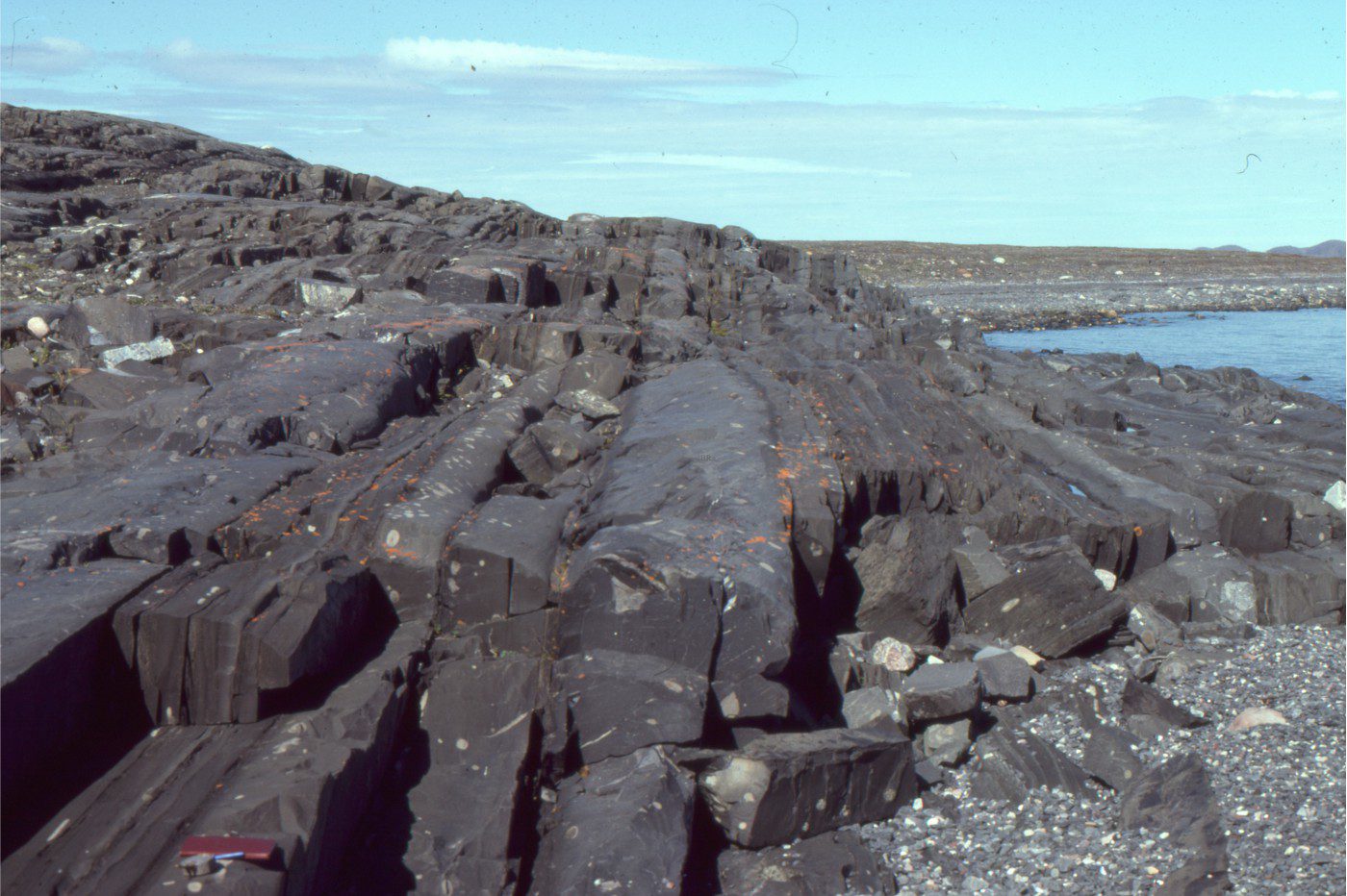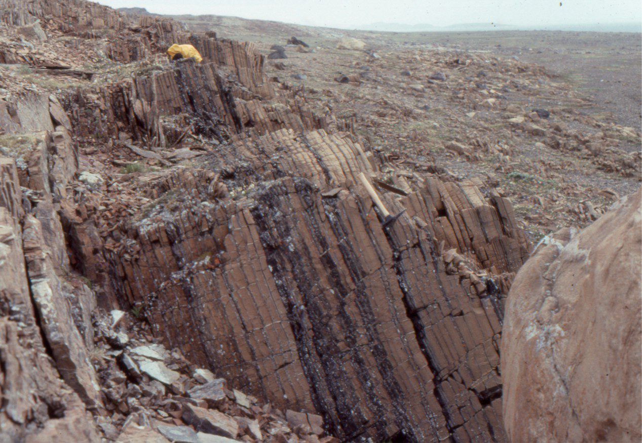
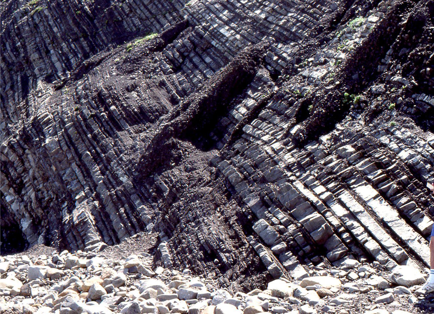
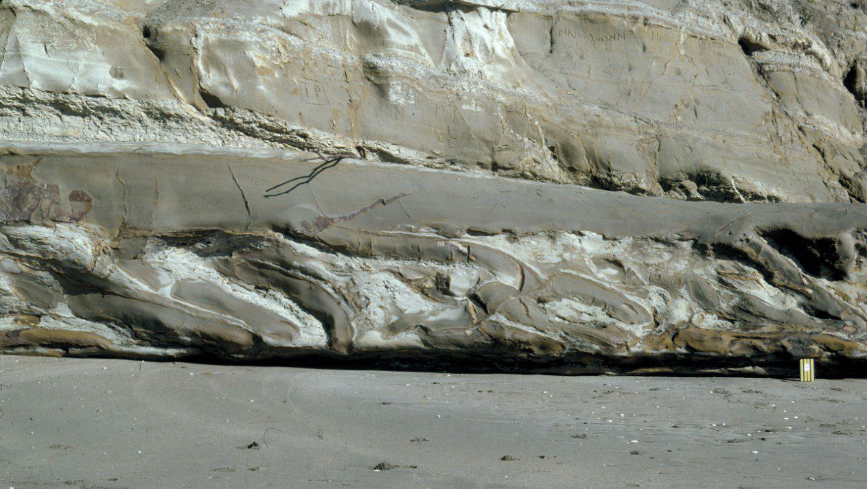
Parallel bedding in a Paleocene turbidite succession, Point San Pedro, California. The thickness of individual beds varies little along their lateral extent, at least within the confines of the outcrop; our view of bedding planes is limited to their 2D extent. The thickest bed is about 50 cm. Geologist’s shoe on the bottom right.

The primacy of beds, bedding, and bedding planes

Beds are the fundamental units of stratigraphy and sedimentology. They are the first things we identify and measure in outcrop, core, and borehole geophysical logs. Beds are the foundations of stratigraphic successions.

Etymologically, the words strata (plural) and stratum (singular) predate the anglicised synonym bed. Leonard da Vinci (1452-1519) and Nicolas Steno (1638-1686) made frequent reference to stratum. The word stratification and its variations are derived from this Latin root. The word bed, in the sense of a resting place or dug plot goes back to Proto-Indo-European roots (about 5000 years back). The context of a sea-bed, where things come to rest, derives from the 16^th C Old English bedd. The geological context, as in a stratum, dates from late 17^th C although frequent use in scientific literature probably had to wait for James Hutton’s opus (1788), William Smith’s regional geological maps (1819-1824), and Charles Lyell’s ‘Principles’ (1^st editions 1830-1833).

Definition of bedding

Beds are sedimentary layers. They usually have observable boundaries top and bottom, referred to as bedding planes. These bounding surfaces are either abrupt where the bedding plane is well defined (you can put your finger on it), or gradational where the compositional or textural change from one bed to the next occurs over some thickness of sediment. Bedding planes demark changes in sediment texture, structure, and/or composition that signify a change in the depositional conditions. The upper bedding plane, if preserved intact, represents a depositional surface – a sediment-air or sediment-water interface. Beds form in all types of sediment: carbonate, siliciclastic, volcaniclastic, chemical. Deposition takes place within a broad spectrum of environmental conditions.

Original orientation

Nicholas Steno (1669) introduced the concept of ‘original horizontality’ where the deposition of sediment at its inception (and therefore bed formation) is approximately horizontal. In reality, the original orientation of a bed will be determined by depositional slope, or paleoslope. This orientation may change during burial compaction, disruption and displacement during soft-sediment deformation, or later tectonism.

Measurable quantities of beds

Thickness: Bed thickness is measured between and at right angles to bedding planes. Thickness can vary from millimetres to many 10s of metres depending on the depositional conditions, such as he continuity of sediment supply. For example, slow deposition from suspension in a lake or deep sea can produce millimetre thick laminae, whereas deposition from a debris flow or pyroclastic density current may be metres thick.

Bed geometry: This is usually identified by the 2D and 3D shape of the bedding planes. The scale of observation, particularly in terms of lateral extent, is not codified but is commonly taken to be at least at outcrop scale. As a general rule, bedding is most easily identified at distance from an outcrop – the closer you get, the more complicated it becomes; the point bar deposits shown below illustrate this problem. Common geometric forms include:

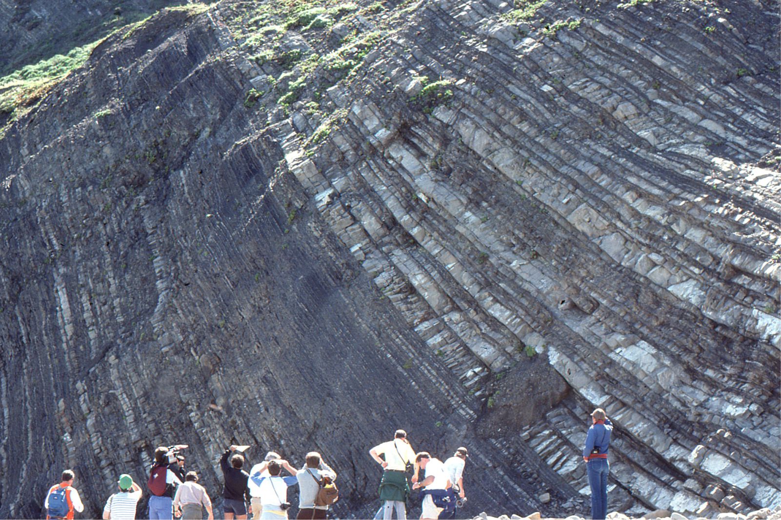
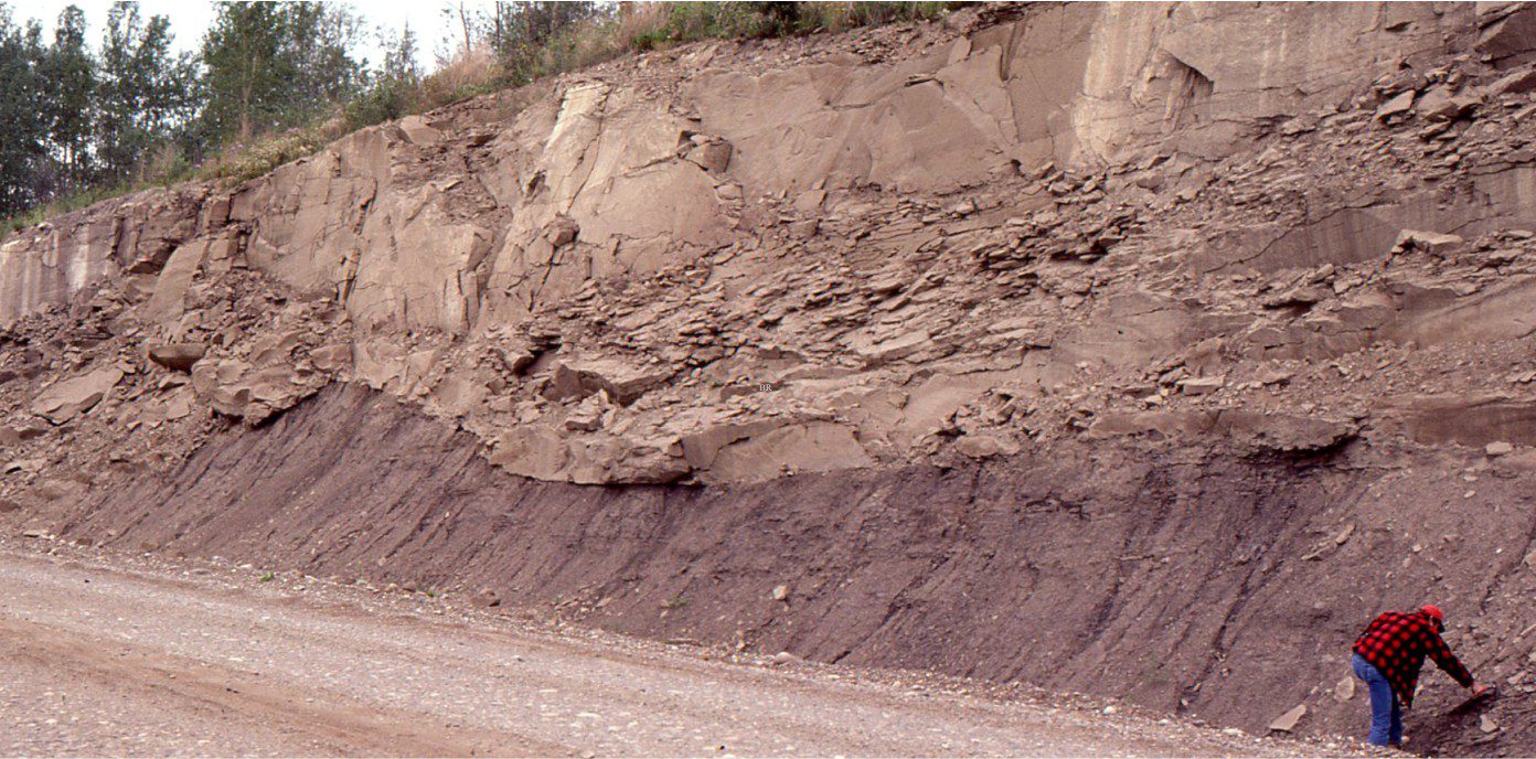
Parallel bedding where bedding planes are parallel at outcrop scale and beyond. Laterally extensive parallel bedding can often be observed in cliff and mountain side exposures. Classic examples occur in flysch-turbidite successions where parallel beds are stacked 100s of metres thick.

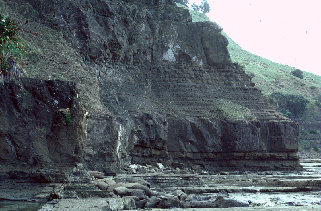
Well-developed parallel bedding in an Early Miocene turbidite-debris flow succession. There is a huge range of bed thicknesses here, from 1-2 cm to about 300 cm. Individual beds can be trace laterally for a few hundred metres. Goat Island Marine Reserve, New Zealand.

Wedge-shaped bedding where bedding planes are not parallel and meet at a pinch out. Theoretically, all beds are probably wedge shaped. At a local scale, examples of this type of bedding include sandstone wedges on a fluvial point bar, and gravel bars in flood-dominated channels on the active portion of an alluvial fan.
Scour shaped bedding: This type is analogous to wedge-shaped beds, but the lower bounding surface is concave upwards. Examples of this type are commonly attributed to channels and channel-forming processes.

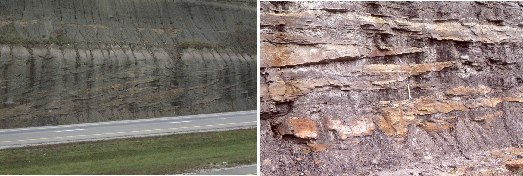
Lateral accretion in this Carboniferous point bar is characterised by discontinuous wedge-shaped sand beds interleaved with siltstone-mudstone layers. From a distance, (left) the inclined lateral accretion beds look quasi-continuous, but their complexity becomes apparent on closer inspection (right). Kentucky, Highway I64.

An amalgamation of sandstone beds filling a fluvial channel – the lowest bed has a distinctive concave-upward bedding plane. Dunvegan Formation (Cretaceous), Alberta.

Internal organization:

Massive bedding – relatively homogenous and structureless throughout.
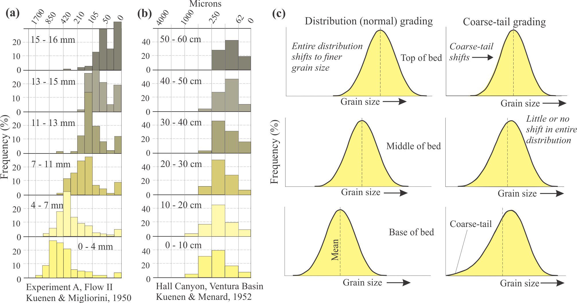
Graded bedding – a change in grain size from bottom to top (e.g., normal, reverse).
Crossbedded – a variety of bedforms are possible depending on sediment grade and current velocity.
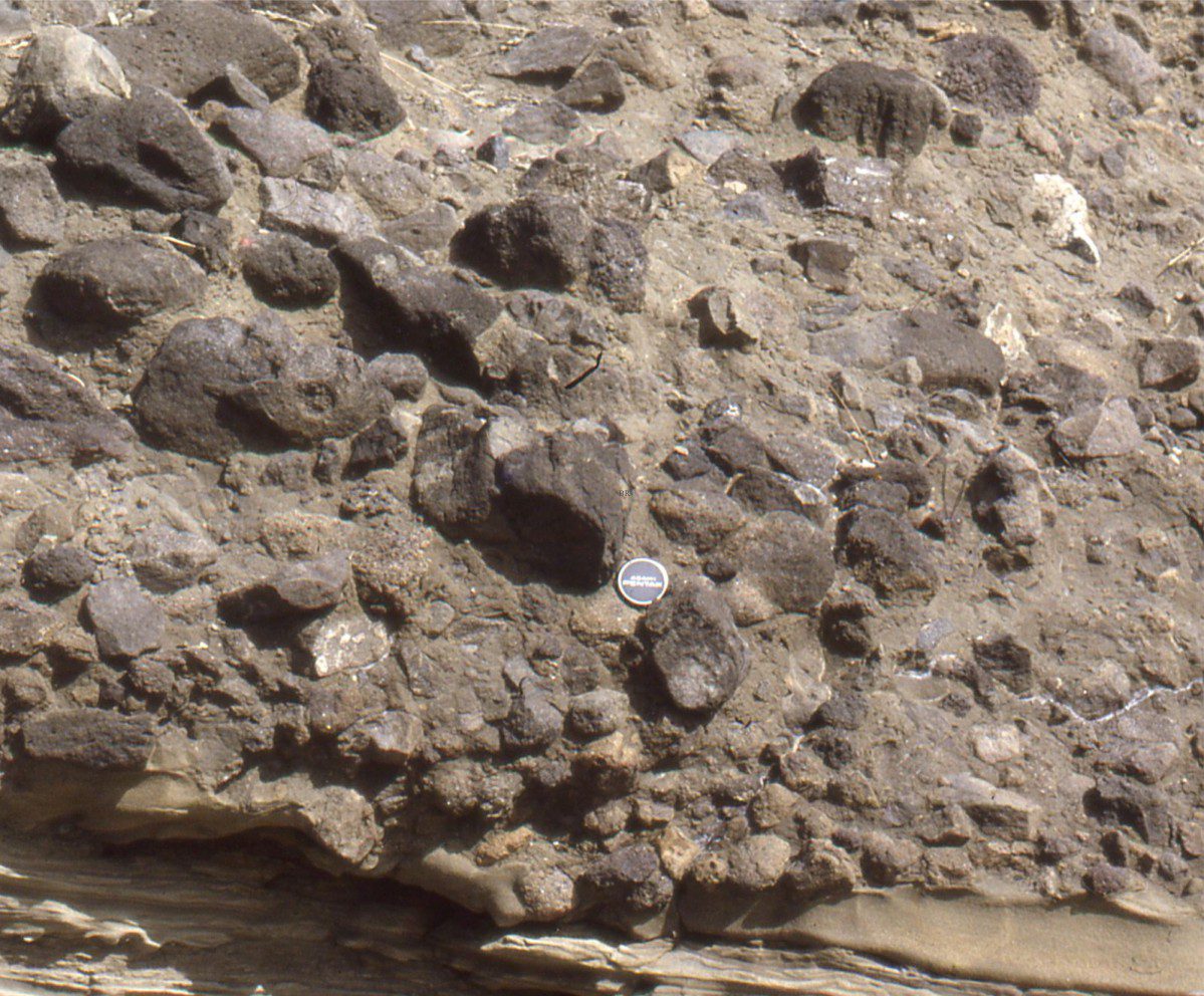
Event beds: Within any succession, there may be beds that stand out because of an abrupt change in thickness, geometry, or composition – they signify a unique event. For example, a succession of bedded sandstone may be interrupted by a bed containing large mud rip-up clasts, signifying an unusual event such as a storm deposit, or beds that record slumping and soft-sediment deformation, or clasts of different composition that may indicate a change in sediment source (provenance).
Marker beds: A bit like event beds except they can be traced over large distances across a sedimentary basin. Common examples are volcanic ash beds that represent single eruptions. Minerals in the ash are also potentially useful for radiometric dating the event. Beds like these are important because they approximate chronostratigraphic surfaces and can be used to correlate widely distributed successions.
Crystal size grading: This applies to chemical sediments. Notable examples include bottom-precipitated evaporite minerals like gypsum and halite, and bedded chert.
The internal organization of all bed types can be modified by bioturbation, compaction, and post-depositional soft-sediment deformation.

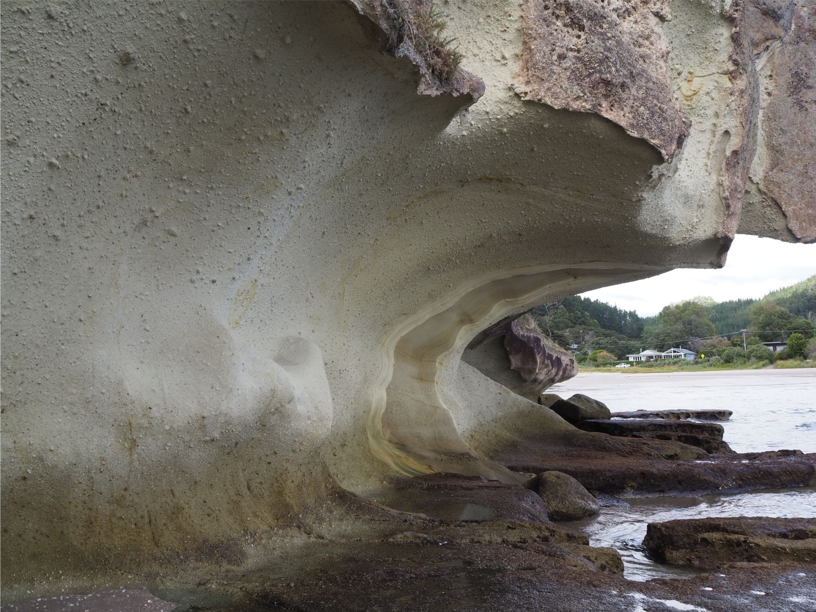
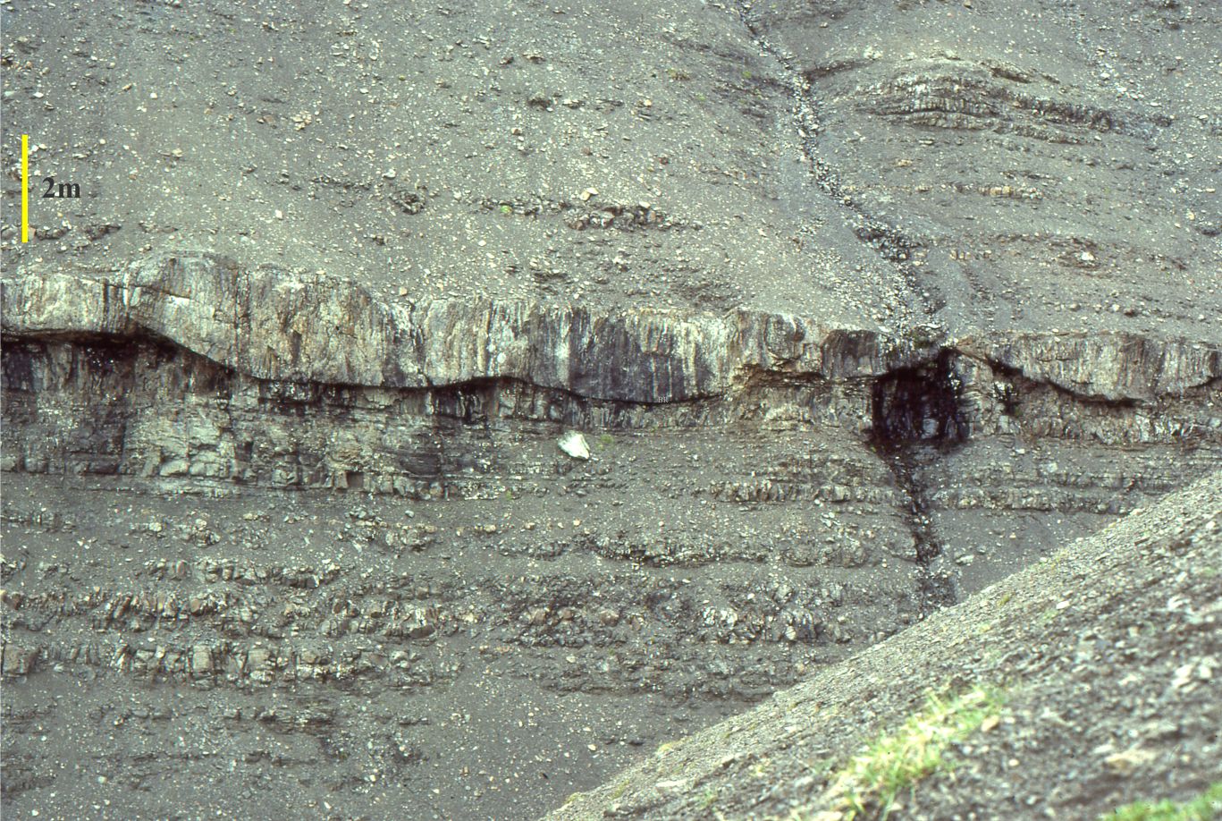
A very distinctive event bed in the Lower Miocene Waitemata Basin, Auckland, consisting of slumped, pulled-apart, folded, and partially liquified sandy turbidite beds. The basal contact is an undeformed glide-plane – a surface over which the entire mass transport deposit moved. The upper bedding plane is irregular, reflecting the relief on top of the slump package, and over which the next sediment gravity flow was deposited.

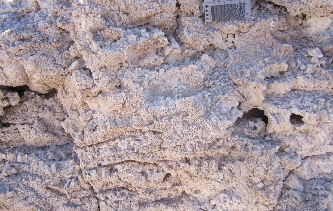
Thin wavy, undulating and discontinuous beds of gypsum that precipitated at the interface between a salt lake (salar) floor and the overlying brine. Each bed is about 20 mm thick. The gypsum crystals grew vertically from the salar floor. Chilean Altiplano. Probably Late Pleistocene.

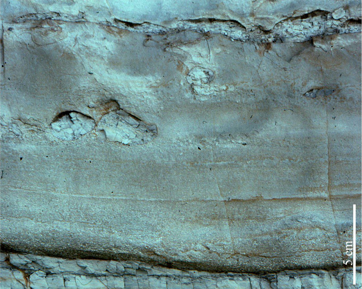
Bedding plane geometry: How a bedding plane is described depends on the resolution of our observations. From a distance, a bedding plane may appear relatively flat or featureless. On closer inspection of the same plane, we might observe undulations that result from large-scale variations in thickness, for example the upper surface of dune bedforms, or large clasts that protrude into the overlying bed; in both cases the departures from ‘flatness’ are produced during the underlying event. However, in many depositional settings, bedding planes are scoured – in this case the scouring is usually associated with the succeeding event. Indeed, erosion and scouring can remove entire beds. Bedding plane irregularities can also result from post-depositional compaction.

The channel-like, lower bounding surface of a crossbedded fluvial sandstone bed has eroded the underlying shelf deposits, in places removing several beds. The fluvial sandstone was deposited during a sea level lowstand when terrestrial drainage extended across the exposed shelf. Jurassic Bowser Basin, northern British Columbia.

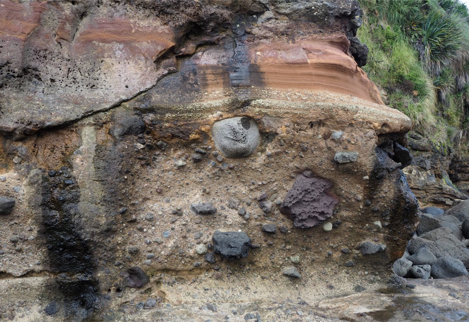
Andesite boulders up to 40 cm across protrude through the upper bedding plane of a lahar where they are draped by later, airfall ash and lapilli (white to red-brown layered beds near the top of the exposure). Pliocene Karioi volcano, Raglan, New Zealand.

The significance of bedding planes

Chronostratigraphic significance of a bed: Every bed represents a period of mechanical or chemical deposition; they are depositional events. The duration of an event can be measured in seconds through millennia. Except under controlled experimental conditions (e.g., flumes), we do not know the duration of these events. We can attempt to find an average duration for a succession, by dividing the number of events (a bed count) by the total time (assuming we can measure the total time represented by the succession), but even this method is woefully inadequate because of…
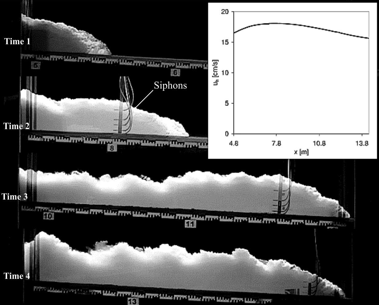
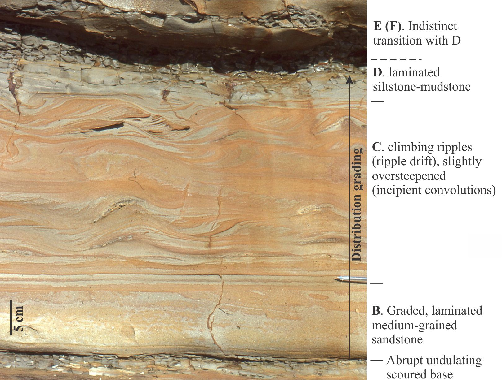
Bedding planes as hiatal surfaces: Bedding planes represent the cessation of depositional events. What is unknown is the length of time between the end of one event and the beginning of the next event. A couple of examples: A bed deposited during a river flood is overlain abruptly by a second, similar bed. Was the second bed deposited during a different period of river flooding, or does it represent a very short- duration shift in depositional locus during the same event (maybe the channel axis shifted laterally, or perhaps there was a surge in flow)? In comparison, turbidity currents leave a well-defined and identifiable depositional record, such as the Bouma sequence. Deposition of coarse-grained intervals (A and B) is probably rapid (minutes, hours, days) but the finer-grained parts of the depositional event may take years to complete. The hiatus between this event and the next could well be measured in 100s or 1000s of years.
Dip and strike: Any description of beds requires us to position them geographically (e.g., latitude-longitude, UTM grids) and to orient them in 3D space. Dip and strike provide unique measures of bed attitude.

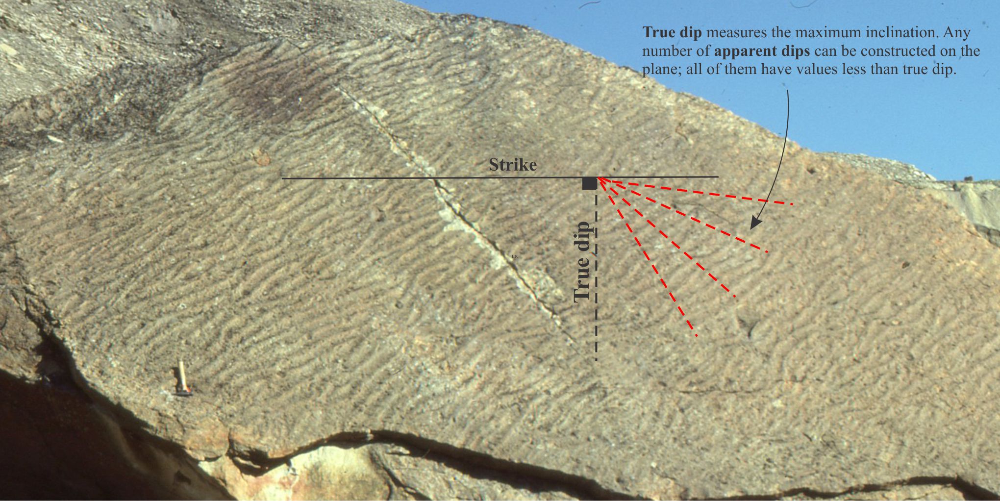
A tilted bedding plane covered with current ripples. The strike, true dip, and apparent dips of are indicated. Paleocene, Ellesmere Island, Arctic Canada.

Things that are not beds

Metamorphic layering: Original bedding can be preserved in low grade metasedimentary and metavolcanic rocks (e.g. subgreenschist to low greenschist grade). High grade rocks (upper greenschist, amphibolite) commonly present compositional layering and through-going foliation that result from alignment of recrystallized sheet silicates like muscovite and biotite. In most cases, original sedimentary bedding has been obliterated.
Igneous dykes (dikes) and sills: Both represent intrusion of igneous melts into an existing pile of rock. They are not beds.
Sedimentary dykes: These too are intrusive bodies (of fluid sediment) that are insinuated into an existing pile of sedimentary beds.
Stratiform iron pans: Bands of nodular limonite and goethite commonly precipitate within existing beds of porous sediment, in response to groundwater infiltration and watertable fluctuations. The iron bands commonly mimic bedding because of the permeability advantage, but can also cross-cut bedding.

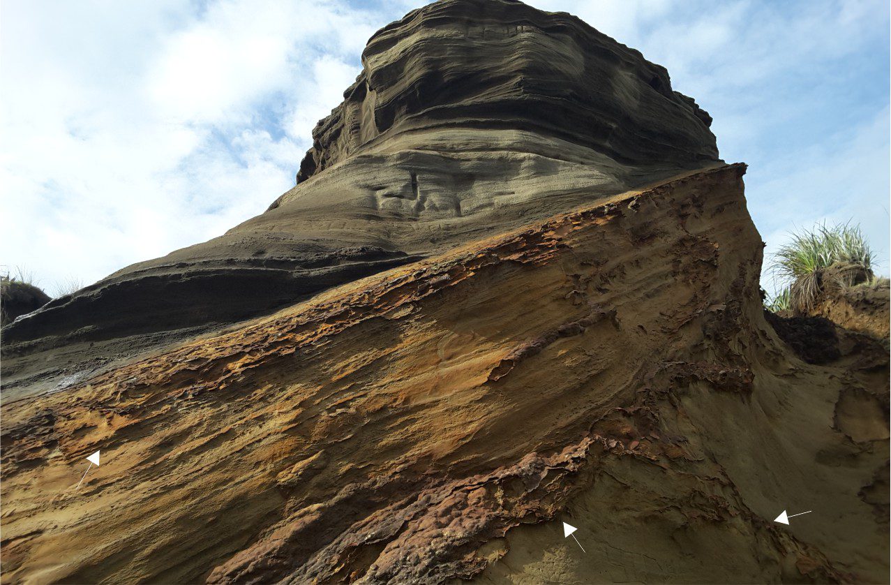
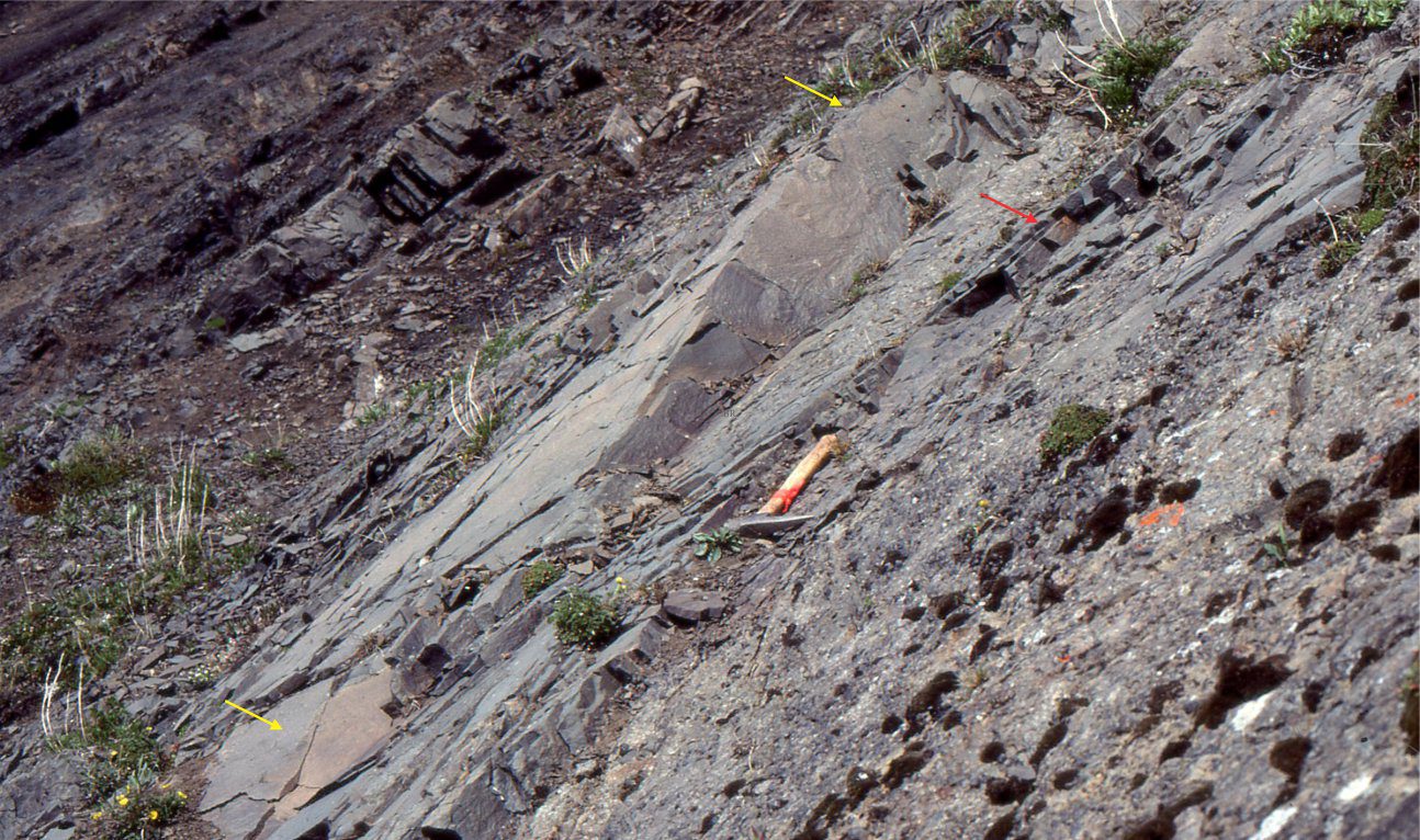
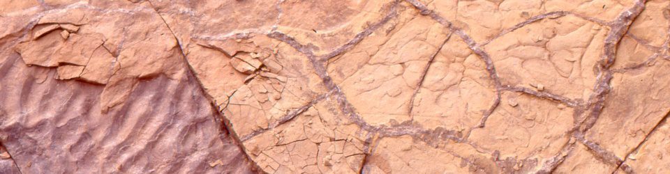
Discontinuous limonite iron pans superficially mimic the left-dipping bedding in these Pleistocene sand dune deposits, but the pans also crosscut the dune bedding (arrows). The iron pans post-date dune deposition and formed as subsurface precipitates of iron oxide during older, fluctuating watertables. Kariotahi, New Zealand.

Salt marsh lithofacies

Leave a Reply

Several generations of salt marsh have formed along Fundy Bay coasts during the Holocene post-glacial, eustatic rise in sea level. At this location the seaward edge is bound by marsh cliffs that define at least three platforms at different elevations, each representing marsh development at different stages of sea level rise. Vegetation here is dominated by Spartina. Small, shallow pannes, or ponds (centre right) are recharged during precipitation and spring tide flooding.

This is the fourth post in a series on vegetated coastal lithofacies – see also:

Seagrass meadows and ecosystems

Seagrass lithofacies in the rock record

Mangrove ecosystems

Mangrove lithofacies

Salt marshes, along with mangrove and seagrass communities, occupy a unique position along many coasts, at the transition from intertidal to terrestrial environments. All three ecosystems also occupy a unique position in the stratigraphic convergence of marine and non-marine lithofacies. The locus of each ecosystem is generally defined as:

Seagrasses occupy intertidal to shallow subtidal zones where there is daily or permanent submergence by tides.
Mangroves thrive in the upper intertidal zone that is regularly flooded by tides, but where the vegetation is not submerged.
Salt marshes occupy a more landward position where they are flooded, but not necessarily submerged, only during spring tides and storm surges.

Modern mangrove and seagrass ecosystems are restricted to tropical – subtropical-temperate latitudes, a situation that appears to have persisted in the rock record. In comparison, modern salt marshes are widely distributed globally, as far north as Greenland and Iceland and south to the Sub-Antarctic Auckland and Campbell islands. Thus, the salt marsh ecosystem may have greater paleogeographic and stratigraphic value.

Salt marsh ecosystems

Like mangrove ecosystems, salt marshes accumulate in low-energy estuaries, embayments and lagoons, and wetland areas behind beaches (the beaches themselves may be high energy, wave dominated but the back-beach area is sheltered). They occupy supratidal zones where seawater flooding only occurs during spring tides and storm surges. Soils are saline, but the degree of saturation alternates from fully saturated during tidal floods, to partly drained and even desiccated during exposure (Allen, 2000). There is little competition from mangroves under these conditions, but at the landward limits of the marshes there is increasing competition from non-halophytic coastal flora.

The most obvious characteristic of salt marshes is their flora, dominated by salt-tolerant (halophytic) plants like Spartina (cord grass) and Juncus, and succulents such as Salicornia. The variation and extent of different plant species depend on temperature and precipitation, the frequency of tidal inundation that also is related to marsh elevation and distance from tidal channels, the degree of desiccation, and soil drainage (Townend et al., 2010, PDF).

Salicornia is a common salt marsh inhabitant. Succulent plants like these are salt tolerant and well adapted to extended periods of soil drying. They also develop dense root tangles that help stabilise the marsh soils.

Sediment infaunal activity can be intense but is restricted to invertebrate species that can tolerate variable salinity and relatively long periods of exposure and potential desiccation. Worms and crabs are most common. Rampant bioturbation by these critters can have a major impact on soil drainage. Foraging birds are common; at some locations grazing by four-legged critters (particularly cattle) can seriously damage the flora and soil structure.

Salt marsh sedimentation

Salt marshes are flat, seaward-dipping platforms that either merge ramp-like with tidal flats or are in abrupt contact defined by micro-cliffs. The marshes are usually transected by branching tidal creek networks that tend to merge seaward to a single waterway. The channels are filled during normal flood tides, but only overtop during spring tides. Channel extent and depth is strongly correlated with tidal range and the magnitude of the tidal prism (the volume of seawater exchanged during a tidal cycle).

Small cliff-like structures are a common feature along the seaward margins of salt marshes. Most are centimetres to decimetres high. They are erosional structures usually associated with marsh retreat.

Allen (2000, op cit.) identified two main types of salt marsh based on sediment composition: organic-dominated and mineral-dominated. Organic marshes derive sediment primarily from local halophytic vegetation; accretion rates in this case are relatively low. Organic matter can accumulate during and between flood events, but it may be subject to aerobic or anaerobic degradation.

Mineralogical marshes derive sediment from the adjacent estuary or lagoon, consisting mostly of mud and silt that is carried in suspension by channel overbank flow; coarser-grained sediment may be introduced to the platform during storm surges. Local ponds, or pannes, dot the marsh surface and may harbour additional invertebrates because of extended periods of inundation. Panne sediment may contain high concentrations of organic matter, including that derived from macroalgae. Prolonged exposure of marshes and pannes can produce a variety of desiccation structures including mud cracks and curled or disrupted microbial mats.

An extensive salt marsh has formed behind coastal dunes near Freeport, Texas. The swaths of Spartina are separated by supratidal, mixed sand-mud flats that are covered by microbial mats in various states of desiccation.

Mineralogical accretion of a marsh only occurs during spring tide inundation. Accretion rate and thickness depend on:

The local accommodation space.
The suspended sediment load concentration.
Proximity to tidal channels and creeks,
The length of time the platform surface is inundated – commonly referred to as the hydroperiod, and,
The settling rate of suspended sediment.

Sedimentation on modern salt marshes is strongly influenced by local vegetation; tidal flow velocities are attenuated by the tangle of plants that trap sediment. Root tangles help bind the sediment. For net accretion to occur, the sedimentation rate during flood tides must exceed erosional losses during the subsequent ebb tides. Salt marsh vegetation can also attenuate storm waves.

Accommodation space

The importance of spring-tide flooding to salt marsh viability means that these ecosystems are strongly influenced by even subtle changes in relative sea level – specifically the dynamic relationship between changes in accommodation space and sediment supply. Such changes may be autocyclic, for example resulting from variations in local sediment supply, local tidal amplification, changes in the tidal channel network, or autocompaction of marsh sediment. Salt marsh platforms will also respond to allocyclic processes such as glacio-eustatic forcing of sea level rise and fall, or basin-wide tectonic subsidence or uplift.

Salt marsh survival based on its response to sea level rise is analogous to that commonly applied to the fate of coral reefs:

Marsh accretion keeps up with sea level rise and is in equilibrium with the creation of accommodation space. Accretion in this context is based primarily on sedimentation rate, but also means that halophytic vegetation must be able to regenerate to maintain the essential character of the salt marsh.
If sea level rise accelerates the marsh will need to catch up. This implies a time lag for sedimentation and regrowth to adjust to the new base level. Recent numerical modelling suggests that this lag may be a few decades (Kirwan and Temmerman, 2009, PDF).
If it is unable to catch up, vegetation will not survive and the marsh will give up.

If sea level rise exceeds the sediment supply rate, then marsh accretion will not keep up. The marshes will eventually drown and, depending on the extent of transgression, may be subjected to ravinement as the shoreline and shoreface shifts landward. Shoreface ravinement has the potential for removal of some or all the salt marsh and associated paralic deposits; the deeper parts of tidal creeks may survive these erosional episodes.

If sediment supply exceeds the rate at which accommodation space is created (i.e., the rate of sea level rise is low, at still-stand, or decreasing), then the marsh will probably expand seaward in concert with the progradation of laterally associated coastal depositional systems (such as mangrove wetlands, lagoon, barrier island, beach, and shoreface).

A swath of beach gravels driven by storms over the adjacent salt marsh. Cobequid Bay, an inlet in Fundy Bay, Nova Scotia. Landward migration of the beach can potentially remove all or some of the underlying salt marsh deposits.

The history of modern salt marshes begins with the post-glacial, eustatic rise in sea level that continued through the Holocene. The global trend in sea level rise will be offset by local or basin-scale differences in subsidence/uplift (particularly the isostatic response to melting ice sheets), local steric effects, sediment supply, tidal amplifications, and storminess. For example, marsh aggradation rates as high as 25.9 cm/century for the past 1400 years have been determined for some Fundy Bay salt marshes, where tidal amplification has been a major forcing factor (Shaw and Ceman, 1999).

Lithofacies associations

Two lithofacies are described: salt marsh and tidal creek. Tidal flats, mangrove wetlands, beaches, and lagoons are important as lateral and stratigraphic associations, but most of these have been dealt with in other posts.

Salt marshes and their deposits rarely occur in isolation – they are usually associated with other paralic depositional settings. Two examples of these facies associations are shown here: Left: Whitford, south Auckland, and Right: Freeport, Texas. Laterally associated lithofacies have the potential to be represented in stratigraphic successions.

Salt marsh lithofacies

In the foreground, Salicornia-dominated, temperate climate salt marsh and intervening supratidal, mud-sand flats. In the background, pale brown sedges have taken over the marsh at slightly higher elevations. Kaiua, Hauraki Gulf, N.Z.

Salt marsh deposits can be thought of as soil profiles – they accumulate mineral sediment and organic matter, they support vegetation, an invertebrate biota and microbiota (e.g., bacteria, fungi), and are subjected to the vagaries of periodic wetting and drying. They consist predominantly of mud and silt, siliciclastic and carbonate, deposited under low energy conditions where intermittent flooding and wave activity are attenuated by the vegetation. The organic content may be concentrated in specific ‘top soil’ layers or distributed through the entire profile depending on sediment supply rates and the duration of the hydroperiod. Like fully terrestrial soils, the plant material is degraded to greater or lesser extents by anaerobic and aerobic bacterial processes, as well as grazing and foraging by invertebrate critters. Wood fragments and the roots of coastal shrubs may also be present, including the roots of mangroves in tropical and subtropical settings.

A 30 cm deep section of salt marsh consisting of silty clay (pale brown) and capping carbonaceous ‘top soil’; the contact between the two layers is gradational. There is no obvious stratification. Root structures from Salicornia and sedges abound. The large holes contain remnants of mangrove roots. Coin (lower left) is 32 mm diameter). Whitford, south Auckland.

A consequence of these depositional conditions is that traction current bedforms are usually absent. Many salt marsh profiles contain little evidence for stratification within depositional units. In others, lamination can develop – good examples from Fundy Bay, identified using X-ray radiography, are illustrated by Dashtgard and Gingras (2005) who interpret the laminae as the products of seasonal variations in sediment supply. The laminae are commonly disrupted by roots and burrows. Laminated muds may develop preferentially in pannes. Pannes that dry out will develop mud cracks and desiccated microbial mats.

Salt marsh profiles may contain multiple episodes of marsh termination resulting from storm flooding or rising in sea levels. Each episode may be bound by:

A low-relief truncation surface (in the case of storm wave encroachment).
Truncation of roots and burrows.
Scattered pebbles or shell lags and lenses derived from laterally associated tidal flats and beaches.
An organic-rich carbonaceous layer where vegetation is re-established.

A 45 cm thick, salt-marsh cliff section reveals stacked marsh-aggradation episodes. Each episode is bound by a thin, dark brown carbonaceous band (white arrows); for each episode the overlying marsh deposits consist of clay and silt. Each episode contains root structures that penetrate the deposits of earlier deposits (e.g., yellow arrow). Larger wood fragments were probably derived from nearby coastal shrubs and trees. Coin (lower right) is 24 mm diameter. Bay of Fundy, Nova Scotia (same locality as shown in the image at top of the page).

Tidal creek lithofacies

A small tidal creek just beyond the downstream limit of salt marsh, Whitford, south Auckland (about 60 cm deep). Ebb tidal flow is from image bottom to top. The sediment here is soft, grey mud that becomes dark green and anaerobic a few centimetres below the surface. The surface is littered with Amphibola crenata gastropods. Burrowing by crabs is intense – also responsible for the mottle appearance of the muds in the exposed creek margin. Small rotational slumps occur on the cut-bank (image centre). Slumped material in the creek bed is gradually dispersed by successive tidal flows.

Tidal creeks that intersect and drain salt marshes receive regular tidal flow but only to bank-full levels during spring tides. Most of the creeks terminate over the marsh surface and there is no continuous through-flow like that in larger tidal inlets and estuarine channels. Consequently, creek sediment is dominated by muds and silts, with the introduction of some sand and gravel during high energy storm events.

Deposition in small creeks, like that shown above, will be dominated by massive or weakly laminated muds and pockets of chaotic blocky muds derived from rotational slumping of creek margins. Burrowing by a variety of invertebrates may completely obliterate any pre-existing sedimentary structures. Roots may extend into the channel margins.

Larger channels show a more diverse array of sedimentary structures including:

Large-scale, shallow dipping laminae consisting primarily of silty muds and thin sandy beds; the dipping beds are analogous to point-bar foresets.
Ripples and small pebble-filled scours.
Thin organic-rich layers, possibly with root structures.
Dipping beds merge with slump packages that form on the steeper cut banks.

A schematic tidal creek profile oriented normal to the channel axis, based partly on the Whitford creek image above, and partly on inference. The dominant lithofacies is clay and silty clay, with some thin sandy veneers along point-bar foresets. The rotational slump glide-planes terminate at the creek floor.

Regular tidal flooding in the creeks means that they can support a more diverse invertebrate fauna – not only burrowing crabs, worms, and shrimp, but also bivalves and gastropods. For example, Holocene creek deposits in Fundy Bay contain passively filled Mya arenaria and Macoma balthica bivalve burrows several centimetres deep. Worms and shrimp can construct more complex U-shaped burrows with meniscate fills and linings (Dashtgard and Gingras op cit.).

Stratigraphic trends

A stratigraphic section through shell-sand tidal flat and overlying salt marsh clay-silt deposits, capped by a plant-rich organic layer. Root structures in the marsh deposits extend into the top of the shell-sand. The marsh also contains simple vertical burrows, probably excavated by crabs. The tidal flat molluscan fauna is dominated by venerid bivalves. The deposit is late Holocene in age. The section is exposed in a dug canal. Whitford, south Auckland.

Salt marshes, like other coastal paralic depositional settings, occur at the intersection between marine shelf or platform and terrestrial environments. Their preservation and stratigraphic representation depend on whether the depositional system is regressive and prograding, or transgressive and retrogradational. A typical stratigraphic profile for normal regression and progradation is shown below.

A typical coarsening-upward lithofacies motif that can develop during normal regression and coastal progradation (deeper shelf not included). The upper part of the column represents common paralic depositional environments at the transition from marine to non-marine conditions, culminating with salt marsh deposits. Shoreface ravinement during transgression may remove all or some of the marsh deposits.

Stratigraphic trends that indicate progradation are commonly represented by coarsening upward or bed-thickening upward successions that record the progression from relatively deep water (for example below storm wave-base) to shoreface, and culminating with the deposits of paralic environments that in this case includes salt marsh. The stratigraphic trend is exemplified by an upward- progression in grain size and bedforms (particularly ripples, subaqueous dunes, HCS) that reflect increasing wave and current energy across the sea floor, and changes in biota – invertebrates and their trace fossil record. Ideally, the upper part of the succession might include evidence for subaerial exposure (e.g. scour surfaces, desiccation structures, beach rock).

[paralic here refers to any depositional system at the junction of marine- terrestrial environments: beach, barrier island, coastal dunes, lagoon, estuary, tidal flat, coastal plain, delta interdistributary bay].

Shoreline retreat during a rise in relative sea level will drive the landward excursion of salt marshes – the survival of the marsh system will depend on whether they can keep up, catch up, or give up as a consequence of inundation. Marsh cliffs will retreat under constant attack by waves. The preservation potential of salt marshes during transgression (like most other paralic depositional systems) is also reduced by erosion beneath the shoreface as it migrates in tandem with the shoreline. Shoreface ravinement can remove all or some of these deposits.

Here’s the link to posts on other lithofacies

Mangrove lithofacies

Leave a Reply

Mangroves dominate this estuarine channel-tidal flat system. The channel is mud-bound, about 1.5 m to 2 m deep and 5 m to 6 m wide, with margins stabilised by the tangle of roots. Tidal flood waters cover the vegetated flats to depths of only a few centimetres. Each tidal cycle replenishes the supply of food and nutrients to the vegetation and the local invertebrate fauna. Whitford estuary, south Auckland.

Mangroves dominate this estuarine channel-tidal flat system. The channel is mud-bound, about 1.5 m to 2 m deep and 5 m to 6 m wide, with margins stabilized by the tangle of roots. Tidal flood waters cover the vegetated flats to depths of only a few centimetres. Each tidal cycle replenishes the supply of food and nutrients to the vegetation and the local invertebrate fauna. Whitford estuary, south Auckland.

This post is part of the Lithofacies Series.

Mangrove trees and forests occupy a very specific zone between fully marine and terrestrial environments in supratidal and upper intertidal realms. They are tolerant of both saline and freshwater conditions but tend to favour the former because there is less competition from terrestrial plants. Their trunks and roots tolerate periodic immersion in seawater (tides), but not permanent subtidal submergence. They prefer low wave- and tide-energy, and muddy substrates; established forests exacerbate the muddiness because they damp waves and tidal flows, and because they add significant quantities of organic detritus to the sediment.

Mangroves are restricted to ocean surface temperatures greater than 15^o C such that their latitudinal extent is about 30^o N and 38^o S. Their tropical to warm-temperate range is reflected in species diversity (greater in warmer environments), and the diversity of associated floral (mostly algal), invertebrate, and vertebrate contributions to mangrove ecosystems. At their southern extent in New Zealand mangroves are represented by a single species – Avicennia marina.

Mangrove evolution

Mangroves are angiosperms. The evolution of angiosperms in the Late Cretaceous is commonly referred to as the Cretaceous Terrestrial Revolution (Benton et al., 2021 OA). This event changed everything – insect evolutionary trends, plant dispersal, a restructuring of the food web and consequent evolution and dispersal of vertebrates and invertebrates, and patterns of sedimentation in environments associated with vegetation. Mangroves, with their specialized adaptations, probably appeared a bit later in the Cretaceous, and may have reached some kind of niche development threshold during the Paleocene-Eocene thermal maximum (PETM), with the appearance of modern genera like Avicennia and Rhizophora. One hypothesis proposes that mangroves developed their tolerance for saline conditions during the PETM when glacio-eustatic sea levels were high and coastal lowlands were inundated. There is evidence that Avicennia grew in coastal wetlands as far north as 75^o N in Siberia and Arctic Canada during this period (Salpin et al., 2019, PDF available). Seed dispersal by ocean currents was probably an important part of mangrove dispersal, but so too were the longer-term plate tectonic changes to continent and ocean configurations with the breakup of Gondwana continuing into the Late Cretaceous and Paleogene, the opening of North Atlantic Ocean and closure of Tethys.

Lithofacies character

Attenuation of waves and tidal currents by mangrove trunks, roots, and pneumatophores results in low-energy depositional conditions dominated by mud and silt, and generally lacking in structures formed by bedload transport of sediment. Any depositional layering will likely be disrupted by growth of roots, pneumatophores, and burrowing by worms, molluscs, and crustaceans (particularly crabs and shrimp). These basic sedimentological characteristics apply to terrigenous- and carbonate-dominated sediments. The organic content of the muds is variable and in outcrop is represented by lithologies ranging from carbonaceous mudstone to coal.

Mangrove wetland substrate is exposed in this tidal channel margin. Except for a few millimetres of grey-brown oxidized mud at the surface, the entire section, about 80 cm thick, is composed of dark blue-grey mud bound by a dense tangle of tree roots and pneumatophores. The root mass helps stabilize the channel bank. The exposed surface is littered with grazing gastropods (Amphibola crenata). Whitford estuary, south Auckland.

Fossil content

A diverse assemblage of benthic invertebrates inhabits the sediment-water interface, burrows beneath its surface, or are attached to exposed roots and pneumatophores. Species diversity is greatest in tropical settings, however, only those with hard shells have the potential for preservation. Crustaceans such as crabs and shrimp and annelids (worms) may leave preservable surface traces or burrows. Crab burrows for example are mostly simple, vertical, passively filled tubes. Shrimp burrows may be Skolithos-like. In New Zealand, nereid worms that are common in coastal wetland muds create U-shaped burrows (Morton and Miller, 1973).

Oysters and mussels that encrust or attach to roots and pneumatophores will probably become detached when either the animal or the woody substrate dies and disintegrates. This may also apply to encrusting foraminifera. Encrusting species like oysters may preserve bioimurred impressions of the wood.

Unfortunately, many of the invertebrates and protozoa that inhabit mangroves also thrive in other intertidal environments. However, mangrove pollen, if preserved, provide unequivocal evidence, particularly when found in association with the other sedimentological features. Mangrove pollen have much greater preservation potential compared with mangrove leaves and wood. Pollen abundance is potentially high in carbonaceous or coaly lithologies. Hisham and Abidin (2023) found this to be the case in Malaysian Early-Middle Miocene coastal wetland deposits, where Avicennia, Rhizophora, and Florschuetzia pollen are abundant.

Despite the abundance of roots in modern mangrove environments, their representation in the rock record is poor. Woody material deposited on the surface is prone to disintegration; in the subsurface it is prone to degradation by anaerobic bacteria. Physical compaction and dewatering during burial will also result in fundamental changes to roots structures. For example, a metre-thick mud when buried 2-3 km will appear in the stratigraphic record as a mudstone only a few centimetres thick. Likewise, compaction of organic rich, coaly layers will reduce original thicknesses by 10 to 20 times. Under these circumstances, the identification of primary root structure is difficult.

A cautionary tale is presented by Perry et al., (2008), who note that encrusting foraminifera, shelly invertebrates, and woody matter that are common in some modern Australian mangrove wetlands, are not preserved in older Holocene deposits – it appears that the carbonate skeletal components may have been dissolved, and that the organic remains altered by aerobic or anaerobic processes.

REDOX conditions

Dig into mangrove wetland muds and you will soon discover the fetid, greenish-black, oozy deposits that are typical of wetlands everywhere. Muds near the surface have varying amounts of oxygen to depths of a few millimetres to centimetres. Below this layer, the low-permeability muds remain permanently saturated and oxygen diffusion is negligible, conditions that promote chemical reduction. There is a progression of redox reactions once oxygen has been depleted, promoted in part by the metabolic activity of bacteria in the muds (Pezeshki and DeLaune, 2012): nitrate is reduced to nitrogen, reduction of manganese (to Mn²⁺) and iron (to Fe ²⁺), sulphate to sulphide (that can combine with Fe²⁺), and CO₂ to methane (hence swamp gas, will-o-the-wisp).

The carbon dioxide component can be generated by anaerobic bacterial breakdown of plant matter, a process that may explain the paucity of fossil mangrove macroflora in the rock record. The lithofacies record of these redox conditions can be preserved as black or bluish- green mudstone-shale in association with carbonaceous or coaly mudrocks. Most invertebrates tend to inhabit the shallowest oxygen-prone deposits.

Excavation by burrowing crabs (arrows) reveals differences in the redox conditions of the substrate. On the left, the excavated sediment on a non-vegetated tidal flat is brownish-grey and much the same colour as the tidal flat sediment. The same species of crab has excavated reduced blue-grey mud in substrates associated with mangrove stands.

Lateral facies associations

Mangrove forests and coastal fringes are bound seaward by intertidal areas – tidal flats in lagoons, embayments (including delta interdistributary bays), behind detached beaches and coastal sand dunes, and the seaward continuation of estuarine channels. Sediment compositions range from mud- to sand dominated, with all manner of combinations in between depending on:

Coastline shape – this is particularly important in seaways having highly embayed and indented coasts, as is commonly the case for drowned valley geomorphic systems and embayments protected by barrier islands and bars.
Tidal range and tidal energy.
The availability of sand.
The capacity for tidal currents and waves to disperse the coarser grain-size fractions, including the capacity for creating ripple and dune bedforms.
The damping effects of seagrass meadows, if present.

Sediment mineralogy can be carbonate- or siliciclastic-dominated, or mixtures of these two. Carbonate intertidal environments commonly contain abundant invertebrate skeletal and calcareous algal fragments, ooids, carbonate mud, microbialites, and detrital gypsum-halite in hypersaline environments. There is a range of sediment bedforms, trace fossils, marine invertebrates, and calcium carbonate secreting algae that provide excellent tools for identification and interpretation of these non-vegetated intertidal lithofacies.

Part of the southern barrier reef on Los Roques Archipelago, Venezuela, emphasizing the back-reef that contains mangroves (Rhizophora mangle) and salt marshes that fringe lagoons with seawater salinities ranging from normal to hypersaline. Sediment beneath the mangroves is anaerobic, and exposed tidal flats commonly develop microbial mats and thrombolites. Distance scale at bottom left is 250 m. Image and information courtesy of José Alejandro Méndez.

In the examples below, the tidal flats are mixed siliciclastic sand-mud with abundant wave and current ripples, and low amplitude bars consisting of disarticulated and fragmented bivalves and gastropods. Seagrass meadows may also be present in intertidal to shallow subtidal environments.

Broad tidal flats develop on the seaward margins of mangrove forests, and in this example, large bedforms include shell banks and bars. The shells are dominated by disarticulated and broken venerid bivalves and subordinate gastropods, all of which have living relatives that inhabit the tidal flats. Other sedimentary structures include a variety of wave and current ripples, and an abundance of crustacean, worm, and mollusc trails and burrows.

The transition from mangrove wetland to fully marine tidal flat lithofacies in this example is distinguished by shell bars, and shell-strewn beaches that are marginal to salt marsh fringes. The abundance of sandy deposits, shelly invertebrates, crustaceans, and bedforms that indicate tidal reversals is in marked contrast to the sedimentological content of mangrove substrates.

Mangrove stands may pass landward directly to terrestrial flora and/or fluvial environments, or to salt marshes that tend to accumulate in upper intertidal to supratidal settings bound by spring tide limits; they are not inundated except at the highest tides. Salt marshes are widely distributed globally, as far north as Greenland and Iceland and south to the Sub-Antarctic Auckland and Campbell islands. Their vegetation is characterised by salt-tolerant succulents like Salicornia and grasses like Spartina (cord grass). Many species of gastropod that graze or scavenge amongst mangroves and tidal flats do not venture into the salt marshes. However, burrowing crabs and worms seem to like this environment and they can be the dominant marine invertebrate there. Salt marsh soils are better drained than their mangrove counterparts with higher concentrations of oxygen. This may be preserved in the rock record as a lateral transition from significantly reduced sediment to more oxidized sediment; stratigraphic profiles will potentially reflect this redox transition.

Salt marsh soils also contain a meshwork of roots of succulents, grasses, nearby mangroves, and other coastal shrubs. Roots have relatively low preservation potential although they may be preserved as carbonaceous outlines or sediment infills. The combination of root growth and invertebrate burrowing means that any primary layering will be disrupted.

A tangle of salt marsh Salicornia roots (fine root structure) interwoven with larger, longer mangrove roots within the salt marsh deposits. In this example there is a significant admix of disarticulated and broken shells near the facies transition with the upper tidal flat. Whitford, south Auckland.

Stratigraphic profiles

A consequence of shoreline excursions during changes in relative sea level is that laterally associated lithofacies will be represented stratigraphically in profiles that record shallowing or deepening upward conditions. This is the essence of Walther’s Law. For example, an ideal shallowing upward, shelf to shoreline profile might show:

At the base of the profile, the transition from mud-dominated outer shelf to sandy inner shelf with bedform indications of wave-base processes, to
Upper shoreface and intertidal depositional conditions.
Regardless of the paleoenvironmental setting, mangrove lithofacies should occur either at the top of the marine stratigraphic succession, or at the transition from marine to non-marine.

How mangroves respond to sea level changes will depend on factors such as

The rate of sea level change. Rapid sea level rise may result in drowning of mangrove stands.
As rates of sea level rise decline, mangroves are more likely to play catch-up of keep-up with the landward-migrating intertidal zone (e.g., Woodroofe, 2018).

When relative sea level falls, the intertidal zone will migrate seaward. The rate at which mangroves will colonize this zone will depend on sediment supply as well as the rate of sea-level change. A good example of rapid shoreward accretion of tidal flats and mangrove development has been documented along the Firth of Thames at the south end of Hauraki Gulf (New Zealand). The coast there in 1950 contained a broad, sandy tidal flat, that by 2007 had been covered by a 1000 m wide band of Avicennia marina; the non-vegetated tidal flat had prograded seaward in response to this floral takeover (Lovelock et al., 2010, PDF available). Shoreline accretion here is largely the result of high sediment flux to the Firth, a consequence of surface runoff from land use changes and deforestation.

Links to the companion posts

Seagrass meadows and ecosystems

Seagrass lithofacies in the rock record

Mangrove ecosystems

Salt marsh lithofacies

Mangrove ecosystems

Leave a Reply

The New Zealand mangrove Avicennia marina fringing the upper limits of tidal flats, interwoven with patches of salt marsh dominated by Salicornia. Tidal flat sediment is a mix of fine-grained sand and mud. The ruffled surface of the flats is primarily the result of burrowing crabs. Hauraki Gulf, New Zealand.

This post is part of the Lithofacies Series.

Manukau Harbour on the west edge of Auckland has several large estuarine inlets fringed by verdant mangrove forests. Residents along one of these inlets, Pahurehure Inlet, considered the mangroves an eyesore and a distraction from the real purpose of the waterway which was to provide easy access for kayaks, sandy beaches, and a safe space for recreation (Stuff report, 2010). After several years of lobbying the local council agreed in 2006 to clear part of the inlet of mangroves, an area of about 11 hectares (Lundquist et al., 2014). What the residents have been left with (as of 2023) is a slough, where thigh-deep anaerobic mud is pock-marked with rotting mangrove stumps, green algal slime, and in places a return of those accursed mangroves. Instead of sandy beaches the estuary is now fringed by salt marsh flora. Though unplanned, the overall result was predictable by anyone with a knowledge of coastal dynamics (tidal currents, sediment budgets and delivery) and coastal ecosystems.

The inner tidal channel and mangrove stump-strewn mud flats of Pahurehure Inlet (near Papakura, south Auckland). Channel depth is about one metre. The inlet margins are now fringed by salt marsh flora dominated by the Button Flower Cotula coronopifolia and a few salt-tolerant grassy sedges, and numerous, young Avicennia marina.

Part of Pahurehure Inlet that was cleared of mangroves (2006-2008) east of the Highway #1 causeway (in the distance, top left). The inlet is drained by tidal channels that are flanked by mud flats. Mangrove stumps abound. In places the mud is thigh-deep; everywhere the mud is anaerobic within a few millimetres of the surface, and unpleasant on-the-nose. The inlet has a typical drowned-valley coastal morphology along the southern margin of Manukau Harbour (west Auckland) and is fed by tidal flows from Tasman Sea.

This is a familiar story along New Zealand coasts where mangroves once thrived – victims of coastal development with its concomitant sediment and contaminant runoff, and folk who need marina access for their boats. Indeed, it is a global story. Mangrove forests are one of the most productive of all marine ecosystems, and one of the most endangered. They are a vital part of the coastal food web, and act as nurseries for all manner of invertebrates, fish, mammals, and reptiles. Mangrove forests perform another vital task – they help to protect coasts because they are very efficient at damping storm-surge waves and currents.

Mangrove distribution

Mangroves have adapted to extreme physical conditions more than any other angiosperm. They grow at the intersection of fully marine and non-marine environments, having adapted to variable salinity and temperatures, tides and wind, storm surges, and soils that tend to be anaerobic.

Mangroves thrive in tropical and subtropical climates along coasts characterized by lagoons, embayments, delta plains, and estuaries. Their ability to grow in saline conditions means there is little competition for this niche from other vascular plants. Their present distribution generally ranges between latitudes 30^o N and S, but in the southern hemisphere their range extends to 38^oS in New Zealand and south Australia because of clement air and sea temperatures (Primavera et al., 2019).

Evolved mangrove morphology

Mangroves grow as trees that, given space, will develop as groves and extensive forests with dense canopies. In the tropics they can grow to heights of 24 m. In some regions, particularly the tropics, the marine wetland forests contain several mangrove species. Two of the most recognizable adaptations are their root systems and an ability to exclude or remove salt from their vascular system (Kathiresan and Bingham, 2001, PDF available).

Root development varies amongst different genera. Avicennia species grow a single trunk that extends directly from the muddy substrate. Its root system tends to be broad and shallow from which grow spongy pneumatophores that extend vertically a few 10s of centimetres above the sediment surface; their primary function is to enhance gas exchange when exposed to air (oxygen, carbon dioxide), and water exchange when submerged. The pneumatophores also provide a substrate for epiphytic algae and diverse invertebrate species.

Left: The distribution of pneumatophores is densest around this mature Avicennia marina trunk. The sediment surface contains a few disarticulated black mussels, oysters, and other bivalves. Sediment composition is about 90% mud. Right: Young mangroves surrounded by pneumatophores attached to the roots of their much older neighbours. Pneumatophores also populate the small tidal channel at image top. Both images from Raglan Harbour, West coast New Zealand.

Rhizophora species have evolved fundamentally different root systems, with spectacular stilt-like structures that raise the main part of the tree above the sediment surface.

The third most common root system is the buttress type where large roots spread radially across the sediment-water interface (e.g., Xylocarpus). This root type stabilizes the tree in conditions where high winds and storm surges are frequent.

Mangrove leaves are thick and leathery. They have evolved the ability to reduce transpiration. Mangroves are angiosperms and produce flowers and seeds (also called propagules). Seed distribution and germination have evolved, like other mangrove traits, to survive saline conditions where dispersal is primarily by wind and tidal currents. Propagules can survive many months in transit to locations where they can put down roots.

An Avicennia marina tree canopy with many fruit buds at different stages of development. When ripe, they fall to the sediment floor and are dispersed by the tides. Right: An Avicennia marina propagule that has been transported several kilometres, eventually stranded on an exposed sandy beach. It is putting down roots, but it’s chances of survival are slim on this storm-dominated coast.

Avicennia marina propagules stranded along high tide lines on a low-energy, mixed mud-sand tidal flat; some propagules are concentrated in clumps of dead seagrass. Complete and fragmented venerid bivalves litter the surface (mostly Austrovenus stutchburyi). The patches of grey mud have been excavated by burrowing crabs. Whitford estuary, south Auckland.

Salt exclusion

Most mangrove species can tolerate a range of salinities, from the barely saline (dilution by fresh water) to hypersaline. They have evolved very efficient processes for water uptake, salt exclusion, and prevention of excessive transpiration. Some species, like Rhizophora filter dissolved salt from soil moisture during uptake of water through their roots. In contrast, species like Avicennia absorb saline soil moisture and excrete the salt through special glands in their leaves (Kathiresan and Bingham, op cit.).

Associated flora

Mangroves have adapted to periodic submergence during tidal cycles, but not permanent submergence. Seagrass meadows are commonly found seaward of mangrove stands but the two do not usually co-mingle, partly because of shading by the canopy, and because there is little water movement where currents are damped by the root tangles.

At latitudes beyond the limits for mangrove growth, the niche is commonly occupied by salt marsh flora and fauna. Salt marsh wetland flora such as Salicornia and Spartina can also compete for space within mangrove belts.

Globally, macroalgae in mangrove wetlands are dominated by red and green species. Their presence and abundance depend on the amount of light that penetrates the canopy, the depth of tidal inundation, degree of desiccation, and salinity. Thus, these species are more likely to thrive near forest edges such as along tidal channel margins.

Associated fauna

Like seagrass communities, mangrove forests act as nurseries and food sources for many invertebrate and fish species, including in more tropical realms commercially valuable species of shrimp and prawn. Mangrove trunks, roots, and pneumatophores provide a reasonably stable substrate for encrusting and attached (epiphytic) invertebrates. Encrusting or cemented species include oysters, barnacles, sponges, and bryozoa. Mussels are attached by byssal threads. However, an overabundance of encrusting forms can also damage or kill trees because they prevent water and nutrient uptake – some species of gastropod will graze upon encrusting organisms.

Left: Avicennia pneumatophores encrusted with small barnacles (Elminius modestus) and some green algae. Right: Pneumatophores heavily encrusted by the small black mussel Modiolus neozelanicus and small encrusting rock oysters (Crassostrea glomerata). The pneumatophores have probably ceased to function efficiently and may eventually collapse under the excess weight. Raglan Harbour, New Zealand.

Most mangrove substrates are muddy and anaerobic within the first few centimetres below the surface. Tidal currents and wave wash tend to be weak. Benthic invertebrates that have adapted to these conditions include a variety of grazing and scavenging gastropods. In New Zealand this group of invertebrates is commonly dominated by crabs, worms, and gastropods like Amphibola crenata and Zeacumantus lutulentus that spend most of their time on the surface rather than burrowing, Wood-boring worms (Teredinids) are capable of significant damage to roots and the lower portions of tree trunks. Zooplankton also proliferate, particularly benthic and encrusting foraminifera, and radiolaria.

Tidal flat muds exposed between stands of Avicennia marina are grazed by abundant Amphibola crenata (gastropod).

Large vertebrates can be prolific in species diversity and numbers. This includes many terrestrial mammals that venture from upland regions, birds, and reptiles including the tropical, more water-prone snakes and crocodilians.

Coastal protection

Mangrove forests provide one of the first lines of defense against storm surges along low-lying coasts (coastal plains, delta plains, estuaries and lagoons) (Temmerman et al., 2023, OA). The degree of storm wave attenuation depends on the density of mangrove tree growth (they usually grow with overlapping canopies), tree height, and the width of the forest belt. Flume experiments, and observations of natural systems indicate that storm wave dissipation also depends on mangrove species, where those that develop stilt roots are more effective at dissipating wave energy. This also applies to the potential reduction of tsunami inundation (Husrin et al., 2012, OA).

Experiments using the genus Rhizophora (that develops stilt roots) show that mangrove stands can reduce storm flood by 50%, and that a belt of trees 80 m wide can reduce wave height by up to 80% (Hashim and Pheng Catherine, 2013, PDF available). These empirical assessments also show a dependency on the severity and duration of storms. The results of these and other studies indicate the value of mangrove replanting in areas where forests have been removed, as a natural and relatively cheap method of coastal protection.

Links to the companion posts

Seagrass meadows and ecosystems

Seagrass lithofacies in the rock record

Mangrove lithofacies

Salt marsh lithofacies

Seagrass lithofacies in the rock record

Leave a Reply

Part of a Zostera marina meadow on sandy tidal flats, Savory Island, British Columbia. Mud content here is <10%. Some leaves are 25-30 cm long. There are a few crustacean or bivalve burrows at left centre.

Some criteria that help us identify fossil seagrasses in the rock record

[This post is a companion to Seagrass meadows and ecosystems]

Coastal seagrasses along with mangrove communities are two of the most productive marine ecosystems in the world. Their primary ecosystem functions have been summarized in a companion post. Despite their importance in modern ecosystems and their presumed contributions to fossil depositional systems, they are poorly represented in the actual rock record. There’s a perfectly logical reason for this – seagrasses are angiosperms, flowering monocotyledons that produce leaves, roots, and rhizomes, all of which are readily biodegradable. Seagrasses have very low preservation potential.

So how is it that seagrass communities are presumed to have been important in Late Cretaceous to Recent coastal paleoenvironments? In a few reported cases there is reasonable direct evidence in the form of leaf-rhizome moulds, casts, and bioimmured fragments. But the main lines of evidence are derived from biofacies associations – the array of epifauna and infauna, motile and sessile invertebrates, protozoa (especially foraminifera), and marine algae (particularly those that secrete calcium carbonate) that indirectly indicate seagrass involvement.

Modern seagrass communities thrive in intertidal and shallow subtidal waters, occurring along most of the world’s coasts from the Arctic-Antarctic circles to the tropics. Species diversity is highest in the tropics. Temperate and cool water coasts have fewer species but those that do exist can develop meadows covering many square kilometres (6 species on the Atlantic and Pacific coasts of Canada; 7 in the Mediterranean, 27 in Australia, and a single species of Zostera along New Zealand coasts). This bioregionalism also means fundamental differences in associated lithofacies and biofacies between tropical and cool-temperate environments.

Infaunal activity in this New Zealand example of Zostera muelleri is dominated by (live) buried bivalves (mostly Austrovenus stutchburyi – yellow arrows) and the topshell Zediloma subrostrata (12 specimens in this view – red arrows). There are a few crustacean burrows. The long-spired gastropod Zeacumantus lutulentus is also common (not seen here); both gastropods are scavengers.

In cool and temperate seas, seagrasses are associated predominantly with heterozoan organisms (those that feed on organic matter), phototrophic algae (such as calcareous red algae) and a variety of invertebrates. These associations exist in the modern tropics (with the addition of calcareous green algae), but they share their habitat with or are marginal to coral reefs. Seagrass communities are also regarded as important components of ramp and platform carbonate factories – primarily because of epiphytic organisms such as encrusting foraminifera, bryozoa, and calcareous red algae, and their function as sediment binders and trappers (e.g., Mazarrasa et al., 2015, PDF).

Recognizing ancient seagrass communities

Most publications that identify paleo-seagrass communities do so using indirect criteria; a selection of these papers is linked herein. In a very few cases there is direct evidence where seagrass leaves and rhizomes are preserved intact or as casts, moulds, or impressions. Reich et al., (2015) provide an excellent review of the criteria for seagrass lithofacies recognition, where the evidence is classified as direct (and reliable), or indirect and less reliable (they use terms like “suggestive” and “weak”). Most of the criteria listed by Reich et al., fall into the indirect categories (see their Table 2) – the criteria tend to be weaker because most of the associated invertebrate, protozoa, and algae biofacies are not unique to seagrass communities.

There are some excellent examples of seagrass leaf and rhizome preservation from the Pliocene of Greece and Canary Islands – examples like this are particularly useful for ‘calibrating’ associated fossil biofacies and lithofacies components for application to the more common circumstance where plant fossils are absent.

The examples listed in the table below (certainly not exhaustive) illustrate the range of lithologies and biofacies associations that are used to infer fossil seagrass assemblages.

A few examples where direct and indirect criteria have been used to identify fossil seagrass assemblages: 1. Collins et al., 2006, PDF; 2. Moisette et al., 2007. PDF; 3. Riordan et al., 2012; 4. Tuya et al., 2017; 5. Brandano et al., 2019; 6. Elsa et al., 2020, OA; 7. Baceta and Mateu-Vicens, 2022, OA.

Direct evidence

Although rare, seagrass leaves and roots are documented as carbonaceous remains and as impressions in silicified sediment in rocks as old as Campanian. They are also recognizable as bioimmured casts and micritic linings. The degree of confidence with these interpretations is boosted if leaves and stem are attached, and where epifaunal organisms such as bryozoa and calcareous algae are preserved on the leaves. However, it is possible to confuse these fossilized forms with other coastal terrestrial plants or marine macroalgae.

Well preserved fossil leaves and rhizomes have been reported from Pliocene deposits on Canary Islands and Rhodes Island, Greece. The Gran Canaria site also contains seagrass seeds of the species Halodule (Tuya et al., 2017). The Rhodes Island site contains fossil Posidonia oceanica and a rich assemblage of skeletal hydrozoans and invertebrates including crustose coralline algae, foraminifera, annelids, gastropods, bivalves, encrusting bryozoans, and ostracods (Moisette et al., 2007).

Bioimmuration

Substratum bioimmuration is the process where the skeletal or encrusting material (commonly calcium carbonate) overgrows another organism. This is particularly important where the substrate is otherwise poorly preserved; for example, plant material or soft-bodied invertebrates. There are a variety of organisms that perform this task – encrusting bivalves such as oysters, bryozoa, crustose calcareous algae, the basal plates of barnacles, and corals. The process has the potential to preserve fine details of the substrate structure – in the case of seagrass, this includes leaf branch nodes, leaf veins, and structures on emergent stems.

Indirect associations

Published interpretations of fossil seagrass communities commonly rely on indirect evidence – the presence (or absence) of associated epifauna on leaves and stems, and infauna that roam, graze, or scavenge the sediment-water interface or dwell within the substrate. Epifaunal and infaunal foraminifera figure prominently in these analyses, commonly in tandem with calcareous algae and bryozoans. Most other invertebrates (e.g., bivalves, gastropods, echinoderms, brachiopods, barnacles, crustaceans) may be important contributors to seagrass ecosystems, but they are not diagnostic as such.

Two structures that improve the confidence with which fossil seagrasses can be identified are:

Hook-like structures formed where the encrusting carbonate extends over a leaf edge – they are best observed in thin sections and polished rock slabs, and
Tubular structures where a leaf or stem is completely encased by the encrusting organism. In this case care must be taken to distinguish the encrusting form from superficially similar structures like Serpulid (worm) tubes.

Foraminifera

Motile (can move under their own steam) and sessile forams are common cohabitants with seagrass and in the rock record are the most common group of organisms taken to indicate fossil seagrass communities. This applies particularly to species that are permanently attached to leaves and stems; common examples include the genera Sorites, Planorbulina, and Gypsina . Encrusting species may be preserved attached or bioimurred to seagrass leaf casts. In most cases, preservation potential is high, but a recurring problem is that most attached species also occur on other substrates (e.g., macroalgae, coralline algae), and motile species like Amphistegina and Elphidium are common in other intertidal and subtidal environments.

Calcareous algae

Red algae commonly attach to or encrust seagrass leaves and exposed rhizomes, as they do on other substrates not associated with seagrasses such as brown macroalgae (common seaweeds), mollusc shells, coral rubble, and rock fragments (e.g., Lithothamnion). Crustose species are more likely to preserve seagrass leaves via bioimurration. Hook-like structures formed at leaf crust-overhangs are commonly identified as seagrass leaf artifacts.

Articulate coralline algae (branched, flexible) are more commonly associated with seagrasses than other non-vegetated environments, but even this association is not exclusive. Articulate species are also more likely to detach from the leaf substrate during deposition. Articulate and crustose calcareous red algae are important in both tropical and temperate-cool environments, but may be subordinate to calcareous green algae in tropical settings (e.g., Halimeda, Penicillus).

Calcareous green algae such as Halimeda and Penicillus are photosynthetic, tropical marine dwellers. They are important contributors to carbonate mud factories. They associate with seagrass communities on carbonate platforms and the shallower margins of carbonate ramps, and with a variety of coral reefs in adjacent lagoons or shallow forereef sites.

A forest of articulate calcareous red algae in which there are a few leaves of Zostera muelleri (arrows). The encrusting oyster at left-center is the species Crassostrea glomerata (New Zealand).

Bryozoans

Platey and leaf-like bryozoa can encrust all manner of substrates – in this case a Zostera muelleri rhizome. A remnant of the decaying rhizome is visible at the base of the encrusting mass; the rhizome extended through the circular opening above – the opening is about 3 mm wide.

Bryozoans are a diverse phylum in many shallow marine environments, a diversity that also applies to seagrass communities where both calcareous and non-calcareous species thrive (>150 bryozoa species are associated with some Mediterranean seagrasses; Reich et al, op cit.). Bryozoans that encrust seagrass leaves tend to be unilaminar and less permanent than species that grow on stems and exposed rhizomes – because of leaf flexibility. Colonies that grow on leaves also tend to expand along the length of the leaf and can completely envelop leaves and stems. There may also be evidence for bioimurration of seagrass leaves and rhizomes by encrusting bryozoa (e.g. Taylor and Di Martino, 2014, PDF).

Other invertebrates (bivalves, gastropods, echinoderms)

Infaunal bivalves in many tropical and temperate seagrass communities include the common suspension and deposit feeders (e.g. Venerids, Carditids, Tellinids, and Nuculids), but most of these species also thrive in non-vegetated shallow marine environments. Likewise, epifaunal communities commonly include oysters and Pectinid species, but these too are wide-ranging in other habitats. The mussel family Pinnidae (fan mussels) are common in seagrass substrates but also extend to non-vegetated environments. A similar situation exists for gastropods, although the species Smaragdia may prefer seagrasses. Echinoderms are common inhabitants of seagrass meadows – some species graze on the leaves – but most extend to other non-vegetated settings.

Dense growth of subtidal, upright blades of Zostera muelleri. A gastropod (possibly Cominella adspersa) is grazing epiphytic algae. Bay of Islands, northern New Zealand. Both photos taken by Aleki Taumoepeau, NIWA, Image courtesy of Fleur Matheson, NIWA.

Trace fossils

Given the biological vitality of seagrass communities in intertidal and subtidal environments, it is not surprising that traces and burrows are common in seagrass substrates – we see this in modern depositional settings and their fossil analogues. Burrowing organisms are numerous in these communities – gastropods and echinoderms, crustaceans (crabs, shrimp, sand hoppers); the traces will reflect their diverse behaviours. Common ichnofauna include Thalassinoides, Ophiomorpha, Skolithos, and Scolicia, However, most of these trace fossils are also common in non-vegetated shallow marine settings, so their potential value as seagrass indicators is limited.

Links to the companion posts

Seagrass meadows and ecosystems

Mangrove ecosystems

Mangrove lithofacies

Salt marsh lithofacies

Seagrass meadows and ecosystems

Leave a Reply

Meadows of the seagrass Zostera muelleri exposed at low tide on tidal flats, Raglan Harbour (west coast, New Zealand). They extend into the adjacent subtidal channel. The substrate is fine-grained sand with 10-20% mud. The surface is littered with the shells of the bivalve venerid Austrovenus stutchburyi, a few Macomona liliana (a Tellinid bivalve), and scavenging gastropods. Meadow coverage in this view is a few hundred square metres.

Seagrass meadows are some of the most productive marine ecosystems in the world.

[This is a companion post to Seagrass lithofacies in the rock record]. Four of the images of New Zealand seagrasses were generously donated by Fleur Matheson, NIWA.

I spent much of my childhood wandering the extensive tidal flats and fishing the estuaries of south Waitemata Harbour, the Pacific-fed waterway that embraces east side Auckland, New Zealand. Amongst the many feathered visitors to the tidal flats (between Howick and Beachlands) were huge flocks of black swans that made yearly sojourns to feed on the seagrass meadows. Then, sometime in the late 1960s – early 1970s the seagrass meadows disappeared, along with the swans, the once vibrant and productive ecosystem a victim of widespread pollution and sediment flux across the entire harbour (caused by coastal development, reclamation, storm water runoff, and fertilizer-herbicide runoff). This is a familiar story along many NZ coasts – a microcosm of the global problem of coastal degradation. Coastal seagrasses along with mangrove communities are two of the most productive marine ecosystems in the world – they are also the most threatened.

A Zostera meulleri meadow gracing the intertidal shore of Whangapoua Harbour, northern Coromandel, New Zealand. Image courtesy of Fleur Matheson, NIWA.

Seagrass communities

Like fields of wheat, submerged seagrass meadows sway with the passing waves and tidal currents. Despite this poetic analogy, the word element ‘grass’ is a misnomer. Seagrasses are monocotyledons, the group of terrestrial angiosperms that develop a single embryonic leaf (dicotyledons develop two embryo leaves). Seagrasses evolved a tolerance to saline conditions from their Late Cretaceous terrestrial ancestors. Like their terrestrial cousins, they develop extensive root systems, produce flowers, and are pollinated while submerged by all the critters that graze, hide, or live within their leafy corridors. Seagrasses are not related to seaweed and other forms of algae – macroalgae are attached by holdfasts rather than roots; algae do not produce flowers. Eelgrass and turtle grass are a couple of common names.

A very nice shot of subtidal Zostera muelleri, swaying in unison with each passing wave. Urupukapuka Island, northern New Zealand. Photo taken by Rohan Wells, NIWA, Image courtesy of Fleur Matheson, NIWA.

Seagrasses have relatively limited species diversity (60 or 72 species world-wide depending on who you talk to) but they are widely distributed across temperate and tropical coasts. Temperate varieties grow in estuaries, bays, and lagoons, forming extensive meadows between mangroves or salt marshes, and the seaward continuation of tidal and subtidal flats. Tropical varieties also grow in these settings including shallow lagoons behind coral reefs. They tend to avoid coasts that are subjected to high energy wave conditions (e.g., open seas surf zones) where substrates are continually reworked. And like mangrove communities, they help protect coastal areas from strong tidal currents and storm wave attack.

Water depths

Seagrasses thrive in waters shallow and clear enough to permit sufficient light penetration (for photosynthesis). Meadows that develop on tidal flats are subject to diurnal submergence. Some species also thrive in subtidal settings, usually limited to the shallowest few metres of the photic zone but they have been found as deep as 90 m. Frequent periodic or continuous submergence is a prerequisite for their survival. A few genera such as Posidonia are restricted to subtidal conditions, others extend across the range of water depths (e.g., Zostera, Thalassia). They prefer substrates that are not continually reworked by strong currents and energetic waves, which means they usually avoid open coasts with surf zones. They also avoid areas subjected to desiccation.

Physical characteristics

Rhizomes, leaves, and roots of Zostera muelleri. Leaf stems and roots can develop on the same rhizome nodes. These specimens are 15 cm long; the leaves have been shortened by grazers.

The most common seagrass morphotypes produce long, narrow, flexible leaves with a longitudinal vein. Eel grass and Turtle grass are of this type. Leaves occur singly or in multiples attached to a rhizome via a papery sheaf. Leaf length is variable among species but commonly is 15 cm and more. Leaf margins are smooth. A few smaller species produce more oval-shaped leaves, each attached by a single stem to a rhizome; other small species are compound with multiple leaves arranged in opposite fashion on a single stem (Morrison et al., 2011, PDF).

Rhizomes have a thick, stringy appearance. They are segmented, separated by nodes from which leaf stems and new rhizomes extend. Much finer roots spread from the rhizomes. Rhizomes spread laterally within the substrate – they are only exposed by erosion or predation.

Seagrass substrates

The following characteristics provide context for fossil substrate lithofacies; most of the data is from Piñeiro-Juncal et al., 2022 (PDF available) who review the physical and chemical properties of seagrass soils.

Dense growth of Zostera muelleri on an exposed tidal flat. The long, skinny leaves are aligned parallel to the direction of the outgoing tidal flow. The substrate here is sandy with 10-20% mud. Ripples that abound on the non-vegetated tidal flats are not present across the meadows because the seagrass has dampened wave and current flows. Small trails (bottom right) were made by the gastropod topshell Zediloma subrostrata.

Seagrass substrates can be classified as marine soils: Although they are not always referred thus in the sedimentological literature, the substrates possess many of the characteristics of their terrestrial soil counterparts – they occur at the sediment-water interface and are subjected to physical, chemical, and biological processes, they are granular, contain organic matter, water, micro- and macrobiota, and gasses (in this case dissolved oxygen and carbon dioxide), and provide the foundation for plant life.
Composition: Seagrasses grow in siliciclastic, carbonate, and mixed carbonate-siliciclastic sediment that is unconsolidated. Carbonate substrates of the tropical kind will potentially contain abundant fragmental reef framework coral, calcareous algae (framework species like Lithothamnion, plus green algae mud producers such as Renalcis and Halimeda), and bryozoan fragments, in addition to diverse invertebrate and protozoa shells and tests. Temperate-cool water carbonate substrates are dominated by non-reef forming invertebrates such as molluscs, barnacles, bryozoa, echinoderms, crustose and articulated calcareous algae, and protozoa such as foraminifera. Most seagrass species are adapted to sandy sediments – measured mud volumes are generally less than 25%. Some species tolerate higher mud contents, others prefer <10-15% mud.
Root zone: Long-lived meadows develop a dense tangle of roots and rhizomes that potentially obliterate all primary sedimentary structures. Compared to seagrass leaves, these root masses have relatively high preservation potential, particularly the thicker more robust rhizomes that may be preserved as casts or molds (e.g., by precipitated iron oxides, calcite, aragonite).
Infaunal burrowing: A diverse benthic fauna will include various invertebrates that crawl or burrow into the root-bound substrate. Distinguishing burrows that have distinct linings, branching, or infill structures (e.g., meniscus structures, or Ophiomorpha nodules) from root-rhizome casts or molds should be relatively straight forward. Simple burrows or trails may be more difficult to distinguish.
pH: Average measured soil-water pH values range from 6.9 and 8.2. A few observations indicate that pH is higher in the upper few centimetres of soil/substrate, becoming more acid below where the rhizome concentration is greatest. The presence of carbonate tends to present higher pH values. Measured organic carbon contents average <2-3%, but range to 10% and more.

Seagrass ecosystem functions

Like mangrove communities, seagrasses are critical components of shallow coastal environments from both ecosystem and human perspectives (in a sense they are the same perspectives). The following functional criteria have been gleaned from Duffy, 2006; Matheson et al., 2009; Morrison et al., op cit; Short et al., 2007, PDF.

The high organic matter production that, during photosynthesis absorbs CO₂, becomes part of the biogeochemical equation of seawater pH buffering. The organic matter also serves as part of the food chain both as live ‘forage’ (e.g., turtles, birds, echinoderms), and as particulate and dissolved components that become part of the food web for reefs, hydrodynamic invertebrate buildups (e.g., oysters), and other seafloor communities.
Sediment substrates are stabilized by seagrass root masses and the leaf clusters help attenuate wave energy and tidal currents. An additional outcome of sediment stabilization and trapping is the recycling of nutrients from plant breakdown, nutrients that are important for seagrass growth.

Dense growth of subtidal, upright blades of Zostera muelleri over a litter of dead leaves, the breakdown of a which provides nutrients to the seagrass meadow and soil microbes. Bay of Islands, northern New Zealand. Photo taken by Aleki Taumoepeau, NIWA, Image courtesy of Fleur Matheson, NIWA.

Seagrass leaves provide a template for epifauna and epiflora (e.g., bryozoa, foraminifera, micro-algae) that become a food source for grazing fish and invertebrates such as crustaceans and gastropods.

Dense growth of Zostera muelleri exposed at low tide. The filigree coatings on the leaves are epiphytic algae that are a food source for a variety of grazing invertebrates. Image courtesy of Fleur Matheson, NIWA.

Dense meadows provide shelter for fish, invertebrates, protozoa (e.g., foraminifera) and commonly act as nurseries for fish, crustaceans such as shrimp, and many species of mollusc, including commercially important species. These nurseries provide protection for juvenile fish, and a platform for fish and gastropod eggs. Neighbouring species groups include polychaetes (worms), echinoderms (grazers), bryozoa and sponges.

Infaunal activity in this New Zealand example of Zostera muelleri is dominated by (live) buried bivalves (mostly Austrovenus stutchburyi – yellow arrows) and the topshell Zediloma subrostrata (12 specimens in this view – red arrows). There are a few crustacean burrows. The long-spired gastropod Zeacumantus lutulentus is also common (not seen here); both gastropods are scavengers.

Fish and invertebrate diversity tend to increase in areas where seagrasses thrive (similar to mangrove communities). Invertebrate diversity is also important because many species will graze macro- and microalgae that compete for the same seagrass niche.
Seagrass leaves on tidal flats are foraged by birds and in subtidal environments by sea turtles, dugongs, and manatees.
Seagrass communities are indicators of environmental health – acting as the ‘canary in the cage’ for eutrophication and pollution of waterways, rising seawater temperatures, and competition for their niche by invasive flora and fauna. There is a well-documented example from the 1930s when an invasive mold pathogen all but eliminated seagrass communities along most North Atlantic coasts (Short et al., op cit.). The disappearance of these communities meant that coexisting ecosystem components such as molluscs and shrimp also disappeared or moved to new neighbourhoods. Invasion of seagrass communities by non-native invertebrates from shellfish aquaculture farming has also been recorded on several British Columbia coasts (Mach et al., 2015).

Link to the companion post

Seagrass meadows and ecosystems

Seagrass lithofacies in the rock record

Mangrove ecosystems

Mangrove lithofacies

Salt marsh lithofacies

Marsquakes: The InSight experiment

Leave a Reply

HiRISE has imaged several recent impacts on Mars surface. This one was acquired on November 19, 2013 – images of the site between 2010 and 2012 bracket the impact timing. The crater is 30 m diameter. Impact resulted in a spectacular ray-like zone of ejecta that spreads up to 15 km from the site and partly covers an extensive sand dune field. Image credit: NASA/JPL-Caltech/Univ. of Arizona

The success of the Apollo lunar seismic experiments (1969 to 1977) provided a real boost to Mars exploration. Exploration of the Martian surface began in earnest in the mid-1970s. The Soviet Union had previously attempted to land two vehicles on Mars in 1971 (Mars 2 and Mars 3). Mars 2 crashed; Mars 3 landed successfully but ceased to operate 20 seconds after alighting, without sending any useful information. However, the two Mars orbiters did continue to acquire images for several months.

Mars exploration continued with NASA’s Viking 1 and 2 orbiters that acquired more than 52,000 images of the martian surface. Both Viking landers successfully alighted the surface about 3 months apart in 1976, Viking 1 at Chryse Planitia, and Viking 2 at Utopia Planitia near the margin of the polar ice cap and 6420 km from its cousin. Both landers were able to sample and chemically analyse air and soil (the first time this had been done) and record various weather parameters. The seismometer on Viking 1 failed to operate. That on Viking 2 functioned for 19 months but because it was located on the lander itself the signal to noise ratio was too low to confidently tease marsquakes from wind-generated signals. However, the lessons learned from these and the Apollo missions were successfully applied to Mars InSight experiments 30 years later.

Mars InSight

(The acronym is easier to remember than its full title – Interior Exploration using Seismic Investigations, Geodesy, and Heat Transport).

InSight landed in Elysium Planitia on November 26, 2018, and deployed its seismometer (SEIS) to the martian surface using a robotic arm. Seismic data was recorded until the operation shut down after December 15, 2022 (because dust on the solar panels had reduced their power output).

SEIS recorded events across a broad spectrum of frequencies which means it could record different kinds of seismic events (marsquakes, impacts), but also had to contend with high frequency wind and thermal noise. Thermal noise is generated from heating and cooling of the surface bedrock and regolith, analogous to that found with the Apollo lunar records. However, the experience with seismic noise gained from both Apollo and Viking 2 experiments allowed seismologists to see through these background signals to tease out the lower frequency signals relevant to Mars internal structure. Signal scattering and seismic coda (a kind of echo or ringing) also tend to mask surface waves – these problems were encountered with the Apollo experiments. Like moonquakes, marsquakes are long lived, continuing for 10 minutes and more because of scattering. In fact, the ringing from one event caused by a meteoroid impact lasted several hours.

InSight’s seismometer (SEIS) was deployed by a robotic arm to sit directly on the martian regolith. The robotic arm covered the tether with a layer of loose soil to protect it from wind-blown sand and to minimize acoustic noise. The dome also acted as a shield against wind and thermal effects. Dome top is about 80 cm high. SEIS weighed 29.5 kg.

Seismic waves

The symptoms of Earth’s indigestion and hiccups are recorded by seismograms as a succession of seismic wave arrivals. Compressional P waves have the highest velocities and are first to arrive – these are the primary arrivals. They are followed by slower secondary shear or S waves. Both P and S waves are referred to as body waves because they are transmitted at depth through a planetary body; it is these signals that provide most of the information on a planet’s deep internal structure. The time delay between the first P and S arrivals is related to the distance to the quake epicenter.

A typical Earthquake seismogram: P-waves arrive first, followed by S-waves. S-waves tend to have lower frequencies than P-waves (more spread out on the graph), but higher amplitude. Surface waves also have the high amplitude and lower frequency than body waves. There can be significant variation on this pattern depending on quake depth, strength, rock composition, and background noise.

P wave deformation is compressional, producing back-and-forth motion at the surface (i.e., motion parallel to the direction of wave propagation). S waves produce up-down and side-to-side motion at the surface (orthogonal to the direction of wave propagation) and tend to be more destructive. S waves are not propagated through fluids (water, gas, igneous melts). Attenuation of S waves at depth in planetary bodies is commonly attributed to a liquid core, or to partial melting in the mantle.

Surface waves confined to the shallow crust comprise a second set of secondary waves that arrive after the body waves (they are slower and have farther to travel). Rayleigh waves produce a rolling ground motion with vertical and horizontal components of movement, and Love waves propagate like S waves but only generate side to side ground movement; they are also attenuated in fluids. Surface waves are most intense following shallow crustal quakes and meteoric impacts; deep quakes produce less intense surface waves.

Marsquakes

More than 1300 marsquakes were recorded over four years of the experiment. Most were of tectonic origin and generated beneath the Martian surface; a few were caused by meteoroid impacts or air bursts. Ninety events having moment magnitudes of 2.5 – 4.2 occurred at teleseismic distances (i.e., distances >1000 km from SEIS).

Two groups of marsquakes have been identified based primarily on frequency: Low frequency (LF) events less than one Hz, and high frequency events (HF) greater than one Hz. HF events are the dominant group and where P and S waves can be identified are attributed to quakes in the crust. LF events usually have recognizable P and S waves and are attributed to deeper quakes. Very high frequency events are mostly caused by thermal responses to diurnal changes in surface temperatures.

Earthquake epicenters can be located accurately because of the large number of seismometers distributed globally. Identifying moonquake epicenters also had the advantage of distributed Apollo seismometer stations. The InSight experiment had only one seismometer such that location of marsquake epicenters required accurate identification of P and S wave arrivals and an a priori seismic model of the martian interior. Note that a general picture of the martian interior (crust, mantle, core) had already been determined from gravity, electromagnetic, and orbital data – what wasn’t known at the beginning of the InSight experiment were accurate depths to the core-mantle-crust boundaries, or the nature of these boundaries.

Signal processing distinguishes between body and surface waves, and between direct P or S waves, and core-reflected and surface-reflected waves. The time delay between P and S waves can be used to estimate to the distance from the epicenter to the seismometer; the same method can also be applied to P and S waves that have been reflected once (designated PP and SS respectively). The modelling process is iterative where both seismic and physical models of the Martian interior are continually updated as the analysis proceeds (for details see Durán et al., 2022, PDF available; and Lognonné et al., 2023, Open Access).

The computed P and S wave velocity-depth profiles are reproduced in the diagram below. Analysis of the low frequency events indicates that their P waves did not traverse deeper than 800 km, much shallower than the expected depth to the core-mantle boundary. S waves on the other hand traversed depths of about 1500 km below which they were strongly attenuated.

However, two notable events in 2021 did produce core-diffracted P waves and surface waves – both were meteoroid impacts (i.e., meteorites or comets) at teleseismic distances from SEIS; both produced large seismic responses with magnitudes >4. The earlier event, S1000a was 7455 km from SEIS and the second event, S1094 was 3460 km (S indicates mission sol, or martian day). Their craters are 130 m and 150 m diameter respectively.

Martian impacts

Six meteoroid impacts or air bursts were recorded by SEIS in 2021, including the S1000a (September 18) and S1094 (December 24) events. Impacts tend to produce relatively strong surface seismic waves, the energy of which depends on impactor size, velocity, and to some extent the obliquity of its trajectory. Two methods of detection and signal analysis have been applied to the martian events:

Surface impacts and air bursts create a fair bit of noise and atmospheric disturbance that produce above-ground acoustic signals. On Mars, these chirps can be recognized for impacts <300 km from the seismometer – at distances >500 km the acoustic signals are dampened by Mars thin atmosphere.
Depending in impact size, a mix of body and surface, direct and reflected seismic waves.

Identification of P and S body waves, and surface Rayleigh waves from the S1094 impact (left) recorded by SEIS December 24, 2021, and S1000a recorded September 18, 2021. Time is in seconds from the first P arrival. Note the long duration post-Rayleigh wave signal run-out to more than 3000 seconds (50 minutes) for S1094 and 3600 seconds (60 minutes) for S1000a. Modified from Posiolova et al 2022 Figures 3 and S1 respectively.

A HiRISE image of the S1094 crater in Amazonis Planitia taken 2-3 Sol after impact. The crater is asymmetric, about 150 m diameter and 21 m deep. Based on empirical models, the impactor was probably 5-12 m across (on Earth it would have burned up on entry). Posiolova et al., (op cit.) calculate the angle of impact at about 30o – the ejecta blanket extends up to 37 km from the crater because of this low angle. White debris in the ejecta is thought to be water ice. Image Credit: NASA/JPL-Caltech/University of Arizona.

The craters from S1000a and S1094 were located by Mars Reconnaissance Orbiter less than 3 Sol after their seismometer recordings (using before and after images of the martian surface). Thus, the impact times and locations are known accurately, providing useful calibrations for marsquake epicenter distance calculations (for example using S-P or SS-PP arrival times). For the two events, the SEIS calculated distance to S1000a was 7591 +/- 1240 km compared with the actual distance of 7461 km; for S1094 the calculated distance is 3530 +/-360 km compared with the measured 3460 km (both differences <1.9%) (Posiolova et al., 2022). The S1094 impact was also notable because it dislodged and scattered blocks of water ice (the bright patches on the image below).

Analysis of the S1000a data indicates P wave diffraction (deflection at a boundary rather than reflection) at a depth between 1500 km and 1600 km (corresponding to a radial distance of 1890-1790 km), that probably corresponds to the core-mantle boundary. The previous P wave depth determined from deep low frequency marsquakes was 800 km (Mars radius is 3,389.5 km measured from the core center).

$Velocity profiles computed for the S1000a impact show both P and S waves transmitting to 1500-1600 km depth. Light red and blue envelopes include the actual impact seismic data; darker colours define envelopes for velocities calculated from other geophysical parameters. The grey envelopes indicate data from low frequency marsquakes – for these events there are no records of P waves transmitting deeper than 800 m. The ray path map (top right) shows direct (P, S) and reflected (PP, SS) body and surface waves for the S1000a impact and a few low frequency marsquakes. The S1000a P wave was a direct arrival at SEIS although it was diffracted by the core-mantle boundary. Modified from Durán et al., op cit, Figures 3A, 3C.$

Velocity profiles computed for the S1000a impact show both P and S waves transmitting to 1500-1600 km depth. Light red and blue envelopes include the actual impact seismic data; darker colours define envelopes for velocities calculated from other geophysical parameters. The grey envelopes indicate data from low frequency marsquakes – for these events there are no records of P waves transmitting deeper than 800 m. The ray path map (top right) shows direct (P, S) and reflected (PP, SS) body and surface waves for the S1000a impact and a few low frequency marsquakes. The S1000a P wave was a direct arrival at SEIS although it was diffracted by the core-mantle boundary. Modified from Durán et al., op cit, Figures 3A, 3C.

Mars internal structure: Velocity-depth profiles

Regolith

Data for the upper few decimetres of relatively unconsolidated regolith was generated from impacts used to drive a heat probe into the soil. Conversion of signals indicates seismic velocities for P waves of 0.098 to 0.163 km/s, and for S waves 0.056 to 0.074 km/s through the uppermost 30 cm of regolith beneath InSight (Lognonné et al., op cit).

Crust

Crustal thickness beneath InSight is about 40 km; the base is indicated by an abrupt increase in both P and S wave velocities. Velocity profiles indicate at least two discontinuities within the crust: one at 8-11 km, above which S wave velocities are 1.7 – 2.1 km/s and P wave velocities are 2.5 – 3.3 km/s, corresponding to basalt with 7-10% unfilled porosity (primarily vesicles). The second discontinuity occurs at 20 +/- 5 km. Thus, the data indicates a 3-layered crust. The global Mars average crustal thickness determined from orbital gravity and topography is 30-72 km Lognonné et al., op cit).

Core-Mantle

The conclusion that Mars core is iron-rich is based primarily on bulk density, gravity and orbital data. Various geophysical, seismic, orbital moments models have been used to calculate the core radius and core-mantle boundary (discussed in some detail by Lognonné et al., op cit). There is reasonable consensus that the core-mantle boundary is between 1,500 and 1,600 km depth, corresponding to a core radius of 1,890-1,790 km. P waves from meteoroid impacts S1000a and S1094 confirm this boundary depth, a depth that also corresponds to significant attenuation of shear (S) waves.

There is a P and S wave discontinuity at about 1,100 km depth that may correspond to a mantle mineral phase transition and an increase in mantle density. This boundary may be analogous to mineral phase – density transitions determined for Earth’s mantle, for example in olivine or perovskite (also common minerals in chondritic meteorites). Average core density is about 6,000 – 6,300 kg/km³.

There is still debate about the structural aspects of Mars’ core. Does it have a solid inner core and molten outer core (S wave behaviour indicates likely melting at the core-mantle boundary) or is the entire core liquid? Le Maistre et al., (2023) argue the latter based on detailed measurement of Mars rotation using InSight RISE data (Rotation and Interior Structure Experiment), demonstrating a rotational wobble that is best explained by a liquid core. The core radius in their calculations is 1,835 ± 55 km, and the bulk density is 5,955–6,290 kg m⁻³ corresponding closely to the values obtained from seismic and other geophysical data.

Unlike Earth, there is no evidence for rotation of Mars outer core. As a consequence, Mars has no geomagnetic field to shield it from solar and cosmic radiation. Given the almost overwhelming sedimentary and geochemical evidence for ancient seas and lakes on Mars surface, Mars atmosphere must have been significantly denser than at present (Mars present atmospheric pressure is less than 1% of Earth’s at sea level) and it is likely that core conditions were very different in the past. Stripping of Mars’ atmosphere by solar winds was probably a direct result of the slow down of core rotation and consequent loss of its geomagnetic shield.

Graded-bedding lithofacies

Leave a Reply

Controlled experiments on turbidity currents allow us to observe the dynamics of flows and the organization of their deposits. Phillip Kuenen and Carlo Migliorini (1950) conducted experiments like the one shown here – they were able to reproduce the kind of graded bedding observed in many outcrops, setting in motion a scientific rethinking of deep-sea sedimentary processes that still resonates today.
The experimental flow shown above was designed to sample the concentration of sediment suspended in the turbulent plume over the duration of the flow (using siphons). Four time-lapse images show different stages of flow development, with two of the siphons at 8 m and 11.6 m from the flume inlet. The inset curve plots flow velocity with distance along the flow path. Image credit: Modified slightly from O.E. Sequeiros et al., 2009. Figure 5, Experimental study on self-accelerating turbidity currents. J Geophysical Research; Oceans

Historical context

The name graded bedding was coined by E. Bailey in 1930 to describe the gradual, vertical change in grain size within a depositional unit (a bed), from coarse-grained at the base, to fine-grained at the top. To comply with his definition, Bailey insisted that the grain size transition should not be interrupted by crossbedding or erosional surfaces. The term could be applied to almost any grain size transition. Bailey surmised that graded bedding formed when sediment was introduced to the water column from volcanic eruptions, dust storms, and river flood plumes, or initiated by earthquakes – the bigger, heavier lumps would fall from suspension fastest, followed by successive deposition of progressively finer material, or from rivers during the waning stages of floods. His interpretations were perfectly reasonable for some examples of graded bedding, like those found in varves, the deposition of air-fall volcaniclastics in water, and from hypopycnal plumes. However, there was one group of rocks for which the explanations offered by Bailey and his contemporaries fell short – the thick, seemingly monotonous successions of flysch.

Flysch, the German word for flow, was applied in the early 19^th C as a stratigraphic descriptor for thick successions of interbedded shale and sandstone (plus a few subordinate lithologies). It was primarily a European term used to describe rocks associated with the Tertiary Alpine Orogeny. Multi et al., (2009, PDF available) provide a nice summary of the history of its usage. A characteristic feature of flysch sandstone beds is their graded bedding; associated lithofacies and sedimentary structures include scoured basal contacts, and finer grained lithologies containing ripples, climbing ripples, and convoluted laminae. Flysch sandstones also tend to be muddy, where the coarsest grain size fractions are mixed with some of the finest grain sized materials (clay, silt), although the proportion of clay and silt increases upwards in each bed.

A thick, seemingly monotonous (really, it isn’t) Paleoproterozoic flysch-like turbidite succession (stratigraphic top to the left). Most beds are graded, and in Bouma model notation contain varying combinations of A, B, C, D, and E depositional units. In this view, the thicker beds also have graded A, B, or A-B divisions. Variations in bed thickness and the proportions of Bouma divisions probably reflect the changing dynamics of active submarine fan lobes. Belcher Islands, Hudson Bay. Field notebook on lower left.

Graded sandstone beds in flysch are repeated in a seemingly endless progression through stratigraphic successions 100s of metres thick. And this was problematic for pre-1950s geoscientists because it required an explanation that provided a mechanism for events repeated 1000s of times – a mechanism that also explained their textural properties. Invoking flood-generated plumes, storm erosion and suspension of sediment, volcanic eruptions, repeated earthquakes, or rapid tectonic uplift and subsidence of a basin floor (a yo-yo like process), didn’t quite meet the requirements. Any of these mechanisms might explain a few depositional events, but not 1000s of them. Likewise, the bathymetry in which they were deposited was also problematic, particularly with the discovery of sand beds in the deep ocean basins, 100s of kilometres from shore; how on Earth did they get there? Enter Phillip Kuenen and Carlo Migliorini (Kuenen and Migliorini, 1950): This duo combined Kuenen’s expertise in experimental sedimentology and Migliorini’s geological field knowledge (Mutti et al., 2009, op cit).

A Paleocene, flysch-like succession of thin-bedded turbidites and mudstones nicely exposed at Point San Pedro, California (top to the right). This exposure is interesting because there are stratigraphic changes in bed thickness: a laminated and rippled mud-dominated package (left) abruptly overlain by three thinning upward sandstone-shale packages (top to the right). The former may represent deposition on the more distal part of a submarine fan lobe (compared with the thick bedded, Paleoproterozoic turbidites shown above); the latter may be the distal fringes of submarine fan lobes, or interchannel overbank deposits.

Although Kuenen and Migliorini are usually credited with introducing the term turbidity current, the existence of density-driven, bottom-hugging sediment-water flows had been known for some time before 1950 and it seems that D.W. Johnson may have pre-empted them in his book The Origin of Submarine Canyons (1939). Density-driven currents had been observed in Lake Mead (reported by Daly, 1936, Gould, 1954 p. 201-207, and others) where they were described as turbid flows, density currents, or gravity-driven flows, mostly generated from plunging sediment plumes (that we would now call hyperpycnal flows). But it was Kuenen and Migliorini’s 1950 paper detailing the proposition that turbidity currents were responsible for the graded beds found in flysch, that set in motion a complete rethinking of deep-sea sedimentation and deep-water depositional processes – so much so that subsequent recording and interpretation of graded bedding has become intertwined with the concept of turbidites and deposition from subaqueous, turbulent density flows.

The Kuenen-Migliorini experiments yielded two notable (and reproducible) results:

Elucidation of the structure and density of the turbulent flows themselves, particularly the dynamics at the flow head, tail, and overlying plume.
The reproduction of graded bedding that proved almost identical to outcrop versions in overall appearance and grain size distribution.

The grain-size distributions for one of their experimental flows are shown below (redrawn from their Figure 5). The histograms represent samples taken at successive distances above the base of the turbidite flow unit. Two observations of note are:

There is a very clear upwards fining trend.
Each sample contains a range of grain sizes that reflects the grain-size distribution of the original sediment slurry.

Normal (distribution) grain-size grading

The kind of grading identified by Bailey (op cit.) and many others since is generally referred to as normal grading or the less common, but more sensible name distribution grading where ‘distribution’ refers to the entire grain-size range. These descriptors distinguish it from two additional kinds of grading – reverse (or inverse) grading, and coarse-tail grading. Sylvester and Lowe, (2004) along with several earlier studies (e.g., Middleton, 1962; Middleton and Hampton, 1976) have shown that grain-size grading trends can change within a single turbidite flow unit, for example inverse to normal grading, coarse-tail to normal grading, or normal to inverse grading. Measures of sorting within a bed can also change in concert with these grading changes.

Examples of measured and hypothetical grain-size distributions in graded beds. (a) Grain-size frequency curves for sampled intervals (in millimetres above base of bed) for one of the experimental flows documented by Kuenen and Migliorini, 1950, Fig 5 (op cit.). The upward fining trend of the entire grain-size distribution is clearly demonstrated; (b) Grain-size frequency curves for a 60 cm thick turbidite bed from Ventura Basin, southern California showing the same kind of fining trend as the experimental turbidite. Curves modified from Kuenen and Menard, 1952, Fig. 1 (Note the different grain-size scale). The outcrop turbidite has a greater range of clast sizes. (c) Hypothetical grain-size frequency curves demonstrating the difference between distribution grading and coarse-tail grading. The former accounts for the entire grain-size range of sampled intervals; the latter only the coarse tail of the curve. Modified from Hiscott, 2013.

Deposition of normal graded beds from turbulent density currents

Typical normal (distribution) grading in the plane-bed laminated B interval of a sandy turbidite. Grains immediately above the slightly scoured basal contact are coarse sand to grit size. The overall fining trend leads to very fine-grained sand near the top of the image. Note the mud rip-up clasts in the Upper part of the unit. From the Lower Miocene Waitemata Basin, Auckland, Aotearoa New Zealand.

Deposition of particles from a turbulent suspension is primarily a function of momentum conservation. Momentum is directly proportional to the product of mass and velocity. As velocity wanes (because of frictional and drag losses), larger grains are deposited on an aggrading bed – this in turn reduces the flow mass and therefore further reduces its momentum. Loss of momentum from sediment dilution is also caused by ingestion of new water at the flow head. Although new sediment can be plucked from the substrate by erosion beneath the flow head, the net effect is a reduction in flow velocity and deposition of progressively finer material.

The sedimentary characteristics of normal grading include:

A gradual, upward change in mean and modal grain-size within a single depositional unit or bed.
Normal grading usually applies to the B, C, and D divisions of Bouma sequences, but may also be present in A divisions (although A divisions are commonly characterized by normal coarse-tail grading).
Grain-size sorting is usually poor at all levels within a bed or flow unit.
Graded beds can be centimetres to metres thick.
Graded beds deposited from turbulent, density currents will tend to be muddy – there is a range of grain sizes at all levels through the bed, but the mud component increases towards the top. The beds commonly have scoured bases.
Normal grading formed from highly turbulent pyroclastic density currents (PDCs), particularly pyroclastic surges (that are a dilute kind of PDC) can include lithic clast sizes ranging from ash to block.
Normal grading can also develop in fluid, gravelly debris flows when there is a component of turbulence in addition to dispersive forces and viscous forces associated with matrix strength.

Distribution grain-size grading in this turbidite (a complete flow unit) begins in the lowermost B interval and ends with the gradational transition from the D to E (hemipelagic) intervals. Both basal and top contacts are scoured. From the Lower Miocene Waitemata Basin, Auckland, Aotearoa New Zealand.

Distribution grain-size grading in this turbidite begins in the lowermost B interval and ends with the gradational transition from the D to E (hemipelagic) intervals. Both basal and top contacts are scoured. From the Lower Miocene Waitemata Basin, Auckland, Aotearoa New Zealand.

Deposition of normal graded beds in still water

Graded beds deposited from settling of sediment suspended in still water (not associated with turbulent flows) tend to be restricted to fine-grained sand, silt, and clay grain sizes. The settling velocities of particles in still water can be estimated using Stokes Law and are a function of grain diameter, particle and fluid density, and viscosity. The general principle here is that larger particles will fall fastest. The finest particles can remain in suspension for days or months. Graded beds formed under these conditions usually lack an eroded base. Examples include varves (seasonal variations in grain-size), deposits from hypopycnal plumes, and hemipelagites on carbonate ramps and continental slopes.

$Paleoproterozoic hemipelagites deposited on a carbonate slope. Each bed shows some degree of normal grading of fine-grained sand to thin laminated shale; the sand-sized fraction is a mix of carbonate (dolomite) and siliciclastic grains. Stratigraphic top is to the right. Costello Formation, Belcher Islands, Hudson Bay.$

Paleoproterozoic hemipelagites deposited on a carbonate slope. Each bed shows some degree of normal grading of fine-grained sand to thin laminated shale; the sand-sized fraction is a mix of carbonate (dolomite) and siliciclastic grains. Stratigraphic top is to the right. Costello Formation, Belcher Islands, Hudson Bay.

Normal coarse-tail grading

The term coarse-tail refers to the coarsest clast sizes on a grain-size distribution curve. Rather than using the entire grain-size range for a deposit, this measure identifies the vertical trend in maximum clast size at successively higher levels within a bed or flow unit (shown diagrammatically in the graphs above). Identification of coarse-tail grading usually requires detailed examination at both outcrop and thin-section/microscope scales (Sylvester and Lowe, 2004 op cit.). It is most easily identified in the A divisions of Bouma sequences where it probably forms by rapid fallout from the suspended sediment load.

Reverse grading

The basal metre of this volcaniclastic, submarine debris flow contains a reverse graded interval above the scoured basal contact – the top of this interval is about the level of the lens cap. From the Lower Miocene Waitemata Basin, Auckland, Aotearoa New Zealand.

Reverse, or inverse grading is usually described as an upward increase in grain-size, and/or the proportion of coarse grains in a flow unit. It is less common than normal grading. It is most easily observed in coarse-grained debris flows where inverse gradation occurs through the entire flow unit (bed), or in the lower part of gravelly or coarse-sand deposits. It has also been observed in turbidites (e.g., Sylvester and Lowe, 2004). Common depositional environments are proximal submarine fans, submarine canyons and slope gullies, alluvial fans, terrestrial landslides and avalanches, and lahars. In pyroclastic density currents there is commonly a combination of reverse grading of pumice fragments and normal grading of denser lithic fragments (Sparks, 1976).

An example of reverse grading of pumice fragments in a thick, non-welded ignimbrite. The curved face of the outcrop is about 2 m high. Clasts near the top of this view are about 8 cm wide; those at the base usually less than 1-2 cm. Late Miocene – Pliocene. Flaxmill Bay, Aotearoa New Zealand.

Reverse grading is far less common in bedload-traction dominated settings (i.e., those not associated with suspended-sediment density flows). Thin reverse graded laminae have been observed in beach deposits where very fine-grained heavy minerals are overlain by coarser, lighter minerals like quartz, feldspar, and bioclastic carbonate fragments – in this case the grading is a function of density segregation during wave swash and backwash.

Two processes are frequently invoked to explain reverse grading:

Debris flow rheology is dominated by relatively high-viscosity mud matrix in which matrix strength plays a key role in the support of clasts. Dispersive pressures that develop during clast collisions are also important in many flows wherein larger clasts, that experience a higher number of collisions, are pushed upward.
Kinetic sieving is the process where fine-grained sediment infiltrates the interstices between coarse framework grains, forcing the coarser material upward (e.g., Middleton, 1970). The process is used at industrial scales (e.g., pharmaceuticals) where coarse materials are separated from fine materials. It may be an effective process for clast separation in the highly agitated environment of a moving debris flow; it has also been reported from grain flows. Kinetic sieving has been proposed to explain reverse grading in some terrestrial avalanche deposits, but in this case some of the fine-grained material is derived by grinding and collision among the larger clasts.

[Middleton G.V. 1970. Experimental studies related to problems of flysch sedimentation. In Flysch Sedimentology in North America, Lajoie J. (ed). Geological Association of Canada: St John’s Canada; 253-272.]

Evolving tempestite lithofacies models

Leave a Reply

Bedding exposure of hummocks and swales (yellow arrows). Hummock amplitude is 15-20 cm and spacing 3-4 m. An underlying swale is indicated by the red arrow. The HCS unit is underlain by a thin pebbly, normally graded sandstone of turbidite character (at the level of the hammer. Mid-Jurassic Bowser Basin, northern British Columbia.

This is the third of three posts on tempestites:

The recognition of hummocky crossbeds by Harms et al., (1975) was an important moment on the time-line of stratigraphic discovery – it conferred empirical status to storm deposits in the rock record. No doubt there had been multiple observations of this bedform by many investigators prior to this publication, loosely described as “wavy lamination”, or “wavy, low-angle truncated laminae”, or “laminae conforming to truncated ripples”, but the significance of its relationship with “strong wave surges” or storm waves required Harms et al., astute theorizing. Decades later, hummocky cross-stratification (HCS) and subsequently swaley cross-stratification (SWS) have become the go-to sedimentary structures for recognition of major storm events in ancient shelf and delta successions.

Most of our knowledge of HCS as a lithofacies is derived from ancient examples, and a few flume experiments (e.g., Dumas and Arnott, 2006). We now know that there is significant variation in the internal stratification and external bedform of HCS. We also know that HCS-SWS are part of a suite of tempestite lithofacies and sedimentary structures that provide evidence for high energy, relatively short-lived events (tropical cyclones, typhoons, hurricanes):

Scour surfaces, lag deposits
Sole structures, including gutter casts.
Density current, turbidite-like deposits.
Other combined-flow bedforms such as modified climbing ripples.
Surfaces that abruptly terminate bioturbation.

Much of our attention on tempestites has concentrated on continental shelves, particularly on the shoreface above storm wave-base. However, storms also influence the depositional and erosional record across environments like deltas, lagoons and tidal flats. In this case, one might expect to find tempestites associated with indicators of tidal currents and periodic exposure.

Two earlier articles on tempestites dealt with the basic forces that act on coastal water masses during storms (Coriolis forces, Ekman veering, Geostrophic flow), and the processes that act on the sediment-water interface to produce a stratigraphic record of these high-energy events – i.e., tempestites.

This post looks briefly at the lithofacies associated with tempestites, presented as diagrams that represent a kind of tempestite interpretation time-line over the last 5 decades. The time-line illustrates some of the changes in our collective thinking about HCS and tempestites as depositional events. I have taken some liberties with these diagrams, adding or subtracting information from the original published examples.

Tempestite lithofacies diagrams and models

Typical external form and internal stratification of HCS; modified from Harms et al.,1975. The basal 1st-order contact is commonly an abrupt erosional surface. The hierarchy of surfaces is from Dott and Bourgeois’ (1982), where 2nd-order contacts separate hummocky lamina sets.

Harms et al., (1975) original diagram showed the basic 3D geometry of surface hummocks and the conforming laminae in 2D profiles. He noted that the laminae have similar geometries in profiles at any orientation, emphasizing the three-dimensionality of the hummocks and intervening swales, in contrast to angle of repose bedforms like tabular and trough crossbeds; this class of HCS is now referred to as isotropic. The diagram also shows truncation contacts between successive, stacked hummocks.

Dott and Bourgeois’ (1982) idealized column incorporates additional lithofacies and sedimentary structures that help a stratigrapher identify tempestites as high energy events:

A basal erosion surface, with or without pebble, intraclast, or shell lags, that commonly preserves a variety of sole structures (e.g., flute and groove casts). The surface probably develops during the waxing stage of storm encroachment.
A hierarchy of depositional and truncation surfaces within the main HCS unit.
Angle of repose crossbeds that indicate a return to traction-dominated deposition.
The succession may be capped by mudstone that contains varying degrees of bioturbation. Mud deposition and cultivation of the infaunal associations are predominantly post-storm.
The abrupt, erosional surface capping the succession signals a new, high-energy event.

An idealized tempestite-HCS lithofacies assemblage, redrawn from Dott and Bourgeois,1982, Figures 3 and 5. The ideal succession includes a basal erosional surface that probably forms during the waxing stage of storm encroachment. The transition from HCS to crossbedded lithofacies that include trough, tabular, and ripple bedforms, indicates waning conditions presaging a return to fairweather, traction-dominated currents. The mudstone likely contains sediment placed in suspension during the storm but deposited long after the storm abates – it may also contain background hemipelagic sediment. Two of the more common variations on the theme identified by Dott and Bourgeois are shown on the right – one where the mudstone is missing (either not deposited or eroded); and an intensely bioturbated section.

The debate over offshore-directed currents versus geostrophic currents received a boost with the paper by D. Leckie and L. Krystinik (1989). They collated paleocurrent data of tempestite-associated facies from several previously published examples, focusing on structures such as sole marks (flute, groove, and gutter casts), parting lineations, oriented wood, combined-flow ripples, and other indicators of slope orientation from HCS and turbidite-like lithofacies. The vector means for each data group were compared with shoreline orientations inferred from lithofacies (e.g., fairweather wave ripples) and paleogeography reconstruction. The data indicates a preponderance of shore-normal, offshore sediment transport, primarily via combined turbidity currents and storm wave oscillatory currents. Notwithstanding later discussions and critiques (e.g., Snedden and Swift, 1990), the Leckie and Krystinik paper continues to serve as a useful tempestite deposition model.

With this diagram I have taken the liberty of extracting a segment of Figure 4 from Leckie and Krystinik (1989) and adding summaries of their paleocurrent data from their Figure 3. The paleocurrent direction for each set of sedimentary structures is presented as the vector mean (arrows), oriented relative to a hypothetical shoreline that was determined from the orientations of fairweather wave-ripple crests. Flute casts and combined-flow ripples allow for reasonably unambiguous paleocurrent determination; groove and gutter casts, parting lineation, and wood orientation are ambiguous indicators of paleocurrents (i.e., their indicated flow directions are 180o apart).

With this diagram I have taken the liberty of extracting a segment of Figure 4 from Leckie and Krystinik (1989), adding summaries of their paleocurrent data from their Figure 3. The paleocurrent direction for each set of sedimentary structures is presented as the vector mean (arrows), oriented relative to a hypothetical shoreline that was determined from the orientations of fairweather wave-ripple crests. Flute casts and combined-flow ripples allow for reasonably unambiguous paleocurrent determination; groove and gutter casts, parting lineation, and wood orientation are ambiguous indicators of paleocurrents (i.e., their indicated flow directions are 180 degrees apart).

Duke et al., (1991) envisage coastal setup driven by refracted, shore-parallel storm waves that increase in power and period as the storm waxes. Return flow generates geostrophic currents that are oblique to the shoreline, currents that interact and combine with oscillatory flow moving sand in suspension and as bedload, depositing flat laminated sand beds (upper flow regime) and HCS. In this model, the strong shore-normal oscillatory flow combines with relatively weak shore-parallel to oblique geostrophic flow. Geostrophic flow extends over most of the shoreface which means that tempestite sand beds are widely distributed across the shelf. Oblique flow is documented by measuring sole structure and sand grain alignment azimuths. Duke et al., maintain that this combination of flow mechanisms is a better explanation for the shelf-wide distribution of tempestite deposits than shore-normal turbidity currents that have more localised distribution.

This diagram has been reproduced almost as is from Duke et al., 1991, Figure 5, except for a few extra labels. The sequence of events over a single storm cycle is represented by:
– Top panel: Lithofacies succession as the storm waxes and wanes. Flat, or plane-bed sand represents maximum shear stress across the sediment bed at the height of the storm, followed by deposition of HCS during combined geostrophic-wave oscillation flow. At a certain point during the waning stage, wave-orbital induced shear stress is not high enough to form combined flow hummocks – at this stage traction current wave bedforms are more likely to form.
– Center panel: The flow velocity profile at the sediment-water interface.
– Lower panel: Flow and bed conditions during the period of the storm.

The Myrow and Southard (1996) paper is still one of the best summaries of storm behaviour, flow conditions in the water column, sediment dispersal, and depositional products across continental shelves, acknowledging shore-parallel, shore-normal, and shore-oblique processes. They also introduce the concept of excess weight force, derived from sediment in suspension, as an important driver of sediment distribution across a shelf during storms (it is a function of density). They stress the importance of sole structures for determining the kinds of paleocurrents that can help distinguish between these three paleoflow directions. Their model diagram introduces a triangular plot that incorporates the most likely combinations of flow types at the sediment-water interface, emphasizing the broad range of sedimentary structures – bedforms, sole structures, and stratigraphic succession during a storm cycle.

Myrow and Southard’s model introduces a tripartite classification of flow types at the sediment-water interface. The triangle apices represent the three fundamental flow types with possible combinations at all other points. It also allows for mapping of pathways as flow mechanisms change during progression of a storm. The diagram is modified from their Figure 7.

Myrow et al., (2002) revamp the ideal tempestite stratigraphic model to include wave modified turbidites, based on Lower Paleozoic shelf deposits exposed in the Antarctic Transantarctic Mountains. Theoretically the model can be applied to geostrophic or shore-normal turbidity currents. The combined flow components include HCS, upper plane bed parallel laminated, and climbing ripple lithofacies. Myrow et al., distinguish these wave-modified climbing ripples from current ripples by their sigmoidal, convex-up foresets – thus they are less likely to have formed by foreset grain avalanching.

A central part of their paper demonstrates the kind of lithofacies variability in offshore to nearshore environments influenced by storms (i.e., event beds), as well as the variability attendant on changing flow conditions during the progress of a storm. Some of these variations are shown below.

Paleocurrent data for the turbidite components includes ripples, parting lineations, and sole structures; the paleoslope was determined from slump fold vergence azimuths. In this model, the turbidity currents moved downslope, driven, at least partly, by excess weight forces generated by resuspension of shallow shoreface sediment by storm-waves and contributions from hyperpycnal flows.

Myrow et al., (2002) idealized tempestite model emphasizes combined flow modification of turbidity currents – i.e., wave-orbital modification (from their Figure 14). The triangular plot (from Myrow and Southard, 1996) maps the transition through the event bed stratigraphy, from purely density current flow to flow combined with oscillatory currents. Myrow et al., also identified several variations on this stratigraphic theme, variations associated with position on the Lower Paleozoic shelf between the paleoshoreline and inferred wave-base (modified from their Figure 7). The main differences in event bed lithofacies are the presence (or absence) of graded or non-graded (massive) sandstones, HCS, upper plane-bed laminated sandstone, and combined-flow climbing ripples, and structures like flute casts and convoluted bedding.

The Dumas and Arnott (2006) model is based on flume experiment observations of the sand-bed response to unidirectional and combined flow. This is an important contribution because it provides sorely needed empirical justification:

The relative contributions of purely oscillatory flow versus combined unidirectional and oscillatory flows during the formation of HCS. They demonstrated that isotropic HCS could form under long period waves with moderate oscillatory flow velocities (0.5 to 0.9 m/s) and weak to no unidirectional flow.
the relative positions of isotropic and anisotropic HCS and swaley bedding (SWS) across the shoreface – the optimal location is between fairweather and storm wave-base where unidirectional currents will be low enough to produce low-angle hummocky laminae.

The experiment-based model presented by Dumas and Arnott (2006, Figure 4B) depicts the relative position of important tempestite bedforms and lithofacies across a shelf, from beach to storm wave-base. The preservation potential of HCS related lithofacies increases beyond the nearshore breaker zone; the potential for HCS preservation in the nearshore is dampened by continual reworking of the sea floor by the turbulence from breaking waves and strong wave-orbital motion.

The tempestite model presented by Jelby et al., (2019) was teased from more than 600 storm event bed in the Lower Cretaceous Rurikfjellet Formation, Spitsbergen. Their model provides a good example of tempestite deposition on a storm-dominated prodelta ramp, where hyperpycnal flows formed offshore-directed, bottom-hugging density currents. An important part of the model also recognises the role of both steady and unsteady wave-generated oscillatory flows, summarized in a 3D triangular plot (a modified version of Myrow and Southard, 1996). They identify 6 basic lithofacies combinations that reflect the relative contributions of the different flow mechanisms – two of the more common lithofacies associations are shown below.

Steady versus unsteady oscillatory flow refers to the degree of continuity of wave periodicity and orbital velocity during the deposition of an event bed. Complex HCS is characterized by abrupt variations in laminae set contacts and thickness, that Jelby et al., interpret as the product of highly variable wave orbitals – perhaps reflecting rapid changes in wind direction, or interfering wave sets.

The lithofacies in this model include most of the bedforms and bioturbation observed in other models: isotropic and anisotropic HCS, combined flow climbing ripples, current and wave ripples, plane bed lamination, scour surfaces, sole structures, graded beds, and various kinds of soft-sediment deformation.

A reorganization of Jelby et al., (2019) Figure 18 showing their modified triangular plot that includes the role of wave oscillation unsteadiness. Two of the more common tempestite lithofacies sections are shown, representing end-member flow conditions (their original figure presents 6 sections, one for each of the main flow domains).

Rationalization of tempestite formation and stratigraphy over the last few decades has concentrated on modern and ancient shelf settings. However, there is increasing recognition that storms also play an important role in the shaping of deltas. The examples presented by Jelby et al., (2019, op cit.) and Vaucher et al., (2023, PDF available) are good illustrations of this role. Lin and Bhattacharya (2021, PDF available) have taken this a step further with their definition of a new class of delta – storm-flood-dominated deltas. Using the Late Cretaceous Gallup Formation as an example, they develop a model delta stratigraphy and diagrammatic reconstruction that incorporates the common tempestite structures, lithofacies, and bioturbation assemblages that are the storm-flood building blocks of delta lobes and prodeltas. The role of hyperpycnal and hypopycnal flows is paramount.

Gutter casts figure prominently in the Lin and Bhattacharya model. Sedimentary gutters are narrow, channel-like, scour-and-fill structures that are common in ancient shoreface and foreshore deposits but have also been reported in deep water successions. The shallow water varieties are commonly associated with storms, but they may also form during fairweather rip-current flow. Gutters can be straight or sinuous in plan-view, with highly variable profile shapes and sizes – widths from centimetres to metres. They are usually oriented normal to shorelines. They are important components of the storm-flood-dominated delta model because of their association with strong, focused, bottom-current flows, and their paleocurrent orientations.

A redrawn (compressed) the storm-flood-dominated delta model presented in Lin and Battacharya (2021) Figure 11 (it's a better fit on screen pages) and included the lithofacies/sedimentary structures listed in Table 1 for each facies assemblage. The upper part of the coarsening-upward succession (delta front, distributary channel) contains mostly traction-dominated bedforms; the lower part (prodelta, storm channel) contains mostly storm-dominated bedforms and stratigraphic surfaces. The model incorporates structures that indicate abrupt, high-energy shifts in depositional style (e.g., abrupt-based sandstone beds that contain gutter casts), and other indicators of storm-influenced deposition – HCS, combined flow bedforms like climbing ripples, and graded beds (particularly in the prodelta sections). The graded beds, common in the prodelta sections, are interpreted as unidirectional hyperpycnal generated flows. Gutter casts figure prominently - five of the more common types of are from their Figure 10.

A redrawn (compressed) the storm-flood-dominated delta model presented in Lin and Bhattacharya (2021) Figure 11 (it’s a better fit on screen pages) and included the lithofacies/sedimentary structures listed in Table 1 for each facies assemblage. The upper part of the coarsening-upward succession (delta front, distributary channel) contains mostly traction-dominated bedforms; the lower part (prodelta, storm channel) contains mostly storm-dominated bedforms and stratigraphic surfaces. The model incorporates structures that indicate abrupt, high-energy shifts in depositional style (e.g., abrupt-based sandstone beds that contain gutter casts), and other indicators of storm-influenced deposition – HCS, combined flow bedforms like climbing ripples, and graded beds (particularly in the prodelta sections). The graded beds, common in the prodelta sections, are interpreted as unidirectional hyperpycnal generated flows. Gutter casts figure prominently – five of the more common types of are from their Figure 10.

Storm surges and tempestites

Leave a Reply

This EUMETSAT / Japanese Meteorological Agency (January 29, 2015) composite image of two tropical cyclones in the Indian Ocean between Madagascar and Australia is a good illustration of the relative sizes of these storms. These two (Diamondra and Eunice) are about 1,500 kilometres apart.

This is the second of three posts on tempestites:

1 Storms and storm surges: Forces at play

3 Evolving tempestite lithofacies models

If there is one suite of sedimentary structures that focuses our attention on shelf or platform dynamics, it is hummocky (HCS) and swaley cross-stratification (SWS). You might be forgiven for thinking that no shelf succession is complete without either or both of these bedforms.

There is consensus that this bedform duo is the product of storms, based on a substantial outcrop database, theoretical considerations (e.g., Myrow and Southard, 1996), and flow experiments (e.g., Dumas and Arnott, 2006), but only a sparse database of bottom-current storm-flow characteristics. They are part of a suite of sedimentary deposits and bedforms called tempestites. They represent depositional events that are distinct from fairweather conditions. There is general agreement that HCS deposits are the product of oscillatory storm-wave orbital bottom currents or bottom-hugging density currents (e.g., turbidity currents) that have been modified by storm waves (i.e., combined flow). Despite these overarching interpretations, the depositional processes responsible for these structures remain a matter of debate (e.g., Duke et al., 1991; Myrow, 2020).

The debate is centred around two important questions:

How is sediment delivered and distributed across shelves and deltas during relatively short-lived storm events. – a question that requires us to evaluate the relative roles of downslope (shore-normal), unidirectional, bottom-hugging currents versus geostrophic currents that flow parallel or obliquely to shorelines?
At the sediment-water interface, what are the relative contributions of storm-wave orbitals and storm-induced unidirectional currents to the development of bedforms like HCS (excluding ambient tidal currents and fairweather along-shore currents)?

Boundary layers in stormy waters

Myrow and Southard’s 1996 elegant description of storm wave and current dynamics is as relevant now as it was nearly three decades ago. An important component of their model deals with the delivery of sediment across a shelf. Ancient tempestite deposits can be 10s of centimetres and even metres thick, which means that substantial volumes of sediment were moved across a shelf during relatively short-lived events. How this is facilitated depends on how energy and shear stresses are partitioned through the water column and at the sediment-water interface, particularly in the bottom boundary layer of shelf and delta water masses.

The diagram below is modified (slightly) from Myrow and Southard (their Figure 1). It shows three distinct layers in waters at average shelf depths within the core geostrophic flow. The location of wave base across a shelf or delta platform is also an important boundary because it limits the depth of wave interaction at the sediment interface.

A surface boundary layer that is maintained by excessive turbulence and mixing. Fine sediment in suspension, for example that derived from wave reworking of the shoreface, or from hypopycnal flows, may reside in this layer for some time and may be deposited long after a storm has ended (which begs the question – should it be included in the definition of tempestites?).
An inviscid middle layer in which viscous forces are small (i.e., Reynolds numbers are relatively high because inertial flow dominates).
A bottom layer where the efficiency of sediment transport depends on two overlapping processes; this layer is where all the sedimentological action takes place:
- A relatively thin layer (centimetres) at the boundary between wave orbitals and the sea floor, where shear stresses are directed alternately onshore and offshore and, because of wave refraction, the motion is normal to the shoreline.
- A thicker layer of unidirectional currents (a few metres) that are directed offshore during intense storms. These bottom currents are the result of coastal setup. They overlap the wave-orbital motion to produce combined flow in the lower layer.

The critical forces at play

The forces that influence sediment transport and deposition in the bottom layer include:

Offshore directed hydraulic pressures, the gradient of which depends on the magnitude of the coastal setup. Coastal setup refers to the elevation of sea level at the coast, where water masses pile up because of wind shear and Ekman Veering of currents that flow at right angles to the wind direction (deflecting to the right in the northern hemisphere). The magnitude of the setup depends on storm duration, wind direction and strength, wave fetch, and the amplifying effects of coastal geomorphology. A seaward pressure gradient develops because the elevated water mass is gravitationally unstable and will tend to dissipate as the storm wanes. Storm cells are also associated with low atmospheric pressures that cause sea levels to rise, but this component only accounts for about 5% of the coastal setup.
Coriolis forces act at 90^o to the wind, deflecting currents to the right in the northern hemisphere. As a storm develops, and depending on the wind direction, Ekman veering will push water masses shoreward and contribute to the coastal setup. Coriolis deflection of the seaward return flow from coastal setup produces isobath-parallel (shore-parallel) geostrophic flow.
Friction forces exist where wave orbitals interact with the substrate. These forces increase from storm wave-base towards the shoreline. Wave orbitals tend to be more symmetrical in deep water, and increasingly elliptical towards the shore (flattened approximately horizontally). Orbital velocities also change with the passage of a storm, as wave heights build over time, but also because winds change direction as cyclonic wind flow passes landward. The magnitude of wave orbital velocity (and therefore shear stress) depends primarily on wave amplitude and period, that also depends on storm duration and fetch.
Sediment suspended in the water column produces what Myrow and Southard call excess weight forces. The concentration of suspended sediment tends to be greatest near the shoreline, decreasing seaward with distance and water depth. Thus, these forces tend to act downslope (seaward). Some of this sediment may be reworked from the sea floor, particularly in the surf zone. However, much sediment is also introduced by rivers and deltas as hypopycnal flows and hyperpycnal flows.

The proportion that each type of force or process influences bedforms and their lateral extent; the thickness of tempestites will vary from place to place and from one storm to the next depending on storm severity, the direction of storm approach along a coast, and coastal geomorphology (e.g., Myrow, 2020, op cit.). Thus, the range of possible lithofacies will also vary from one event to another. Geomorphic systems other than open-ocean shelves, such as large deltas and high-volume rivers, will impact the volume of suspension load and bedload sediment released to adjacent shelves. The response of storm surge encroachment over a delta will also be quite different to that over shelves where river input is minimal; in this case, marine processes will compete with fluvial flood-related processes – recent examples are Bhattacharya et al., 2020, looking at North America delta systems; Vaucher et al., 2023, examining a Late Pleistocene flood delta in Taiwan).

Shore-normal flows or geostrophic flows?

The term “shore-normal” here means bottom-hugging flow normal to shoreline: geostrophic flows parallel isobaths or may be oblique where deflected by seafloor topography. The problems associated with identifying shore-normal or shore-parallel bottom current flows as depositional modes for tempestite deposition is nicely encapsulated by two early publications: Leckie and Krystinik (1989), and Snedden and Nummedal (1991).

Shore-normal flows

Leckie and Krystinik proposed that combined shore-normal density currents (turbidity currents) and wave orbital flows were responsible for the majority of HCS-bearing beds in Cretaceous shelf deposits (Western Canada foreland basin), based on sole mark and parting lineation trends, together with offshore trends in stratigraphic thickness and grain size. Numerous studies have since shown the importance of shore-normal, wave-modified turbidity currents (i.e., combined flow), not only in ancient shelf settings but also across wave-dominated deltas and prodelta slopes where hyperpycnal flows are commonly generated, for example Myrow et al., (2002, Cambrian Shelf – PDF available), Jelby et al., (2019, Cretaceous delta ramp).

Density current flows may be triggered by excess weight forces (noted above), including those generated by plunging hyperpycnal flows, or by resuspension of sediment by storm waves; some excellent examples have been documented in Spitsbergen Cretaceous rocks (Jelby et al., 2019. Op cit.). Zavala (2020, open access) has incorporated HCS in some hyperpycnite lithofacies models.

Geostrophic flows

Storm-generated geostrophic currents develop when Coriolis forces deflect the return flow from coastal setup (the coastal setup pressure gradient is oriented seaward). The interaction of storm wave orbitals with these shore-parallel currents can produce combined flows that parallel or are oblique to the shoreline during the waning stages of storm surging. Snedden and Nummedal (1991, PDF available), while not dismissing the importance of shore-normal processes, made a concerted plug for shore-parallel or oblique geostrophic flows, based on mapping of a distinctive, graded, tempestite bed deposited by Hurricane Carla (1961). Their interpretation was based on measured shore-parallel isopachs and grain size distributions of a storm-deposited sand bed, observed wind forces, and modelled current directions. Likewise, Swift et al., (2006) posit shore parallel storm generated currents to explain bedform, paleocurrent, and sediment distribution in Cretaceous Book Cliff strata (Utah).

Geostrophic flows also interact with waves producing a range of combined-flow bedforms including ripples, dunes, and asymmetrical HCS. However, geostrophic currents are not restricted to the shoreface – they can extend across the shelf beyond storm wave-base where there is no interaction with wave orbitals in the lower boundary layer. In this case, all sediment transport is traction dominated, and bedforms like current ripples, dunes, and lower flow regime plane-bed lamination will form. This suite of bedforms will be coeval with the HCS-dominated tempestites although distinguishing them from other fairweather deposits might be difficult.

Geostrophic flow across continental shelves and deltas tends to be either parallel or oblique to shore, the latter depending on current deflection by shallow bathymetry, and possibly temperature and salinity barriers. Mapped geostrophic flows in modern seas commonly indicate significant departures from shore-parallelism, particularly in deeper waters beyond the shelf break. The example from East Sea (Japan Sea) shows flow vectors (measured, and calculated from sea level elevations) that define several eddies that coincide with seawater temperature anomalies. The eddies are located beyond the shelf-break, but they may complicate flow dynamics across the shelf during storms.

Surface geostrophic currents (black vectors) and sea surface heights (SSH) determined from VISO satellite altimeter data and coastal sea level data for the Sea of Japan between Korean Peninsula and Honshu Island. Sea surface heights are in metres relative to Global Mean Sea Level. The 500 m isobath has been added (black dashed line). Geostrophic currents are mostly coast-parallel across the Honshu shelf but develop 200-300 km diameter eddies farther offshore. UBIM is an ocean buoy. EKWC = East Korea Warm Current. SE = Sokcho Eddy. Image credit: Modified slightly from Son et al., 2014. Honshu I. License CC BY 3.0

Definition of bedding

Original orientation

Measurable quantities of beds

The significance of bedding planes

Things that are not beds

Other posts that introduce basic methods of rock description, mapping, and structural analysis

Share this:

Like this:

Salt marsh ecosystems

Salt marsh sedimentation

Accommodation space

Lithofacies associations

Salt marsh lithofacies

Tidal creek lithofacies

Stratigraphic trends

Here’s the link to posts on other lithofacies

Share this:

Like this:

Mangrove evolution

Lithofacies character

Fossil content

REDOX conditions

Lateral facies associations

Stratigraphic profiles

Links to the companion posts

Share this:

Like this:

Mangrove distribution

Evolved mangrove morphology

Salt exclusion

Associated flora

Associated fauna

Coastal protection

Links to the companion posts

Share this:

Like this:

Recognizing ancient seagrass communities

Direct evidence

Bioimmuration

Indirect associations

Foraminifera

Calcareous algae

Bryozoans

Other invertebrates (bivalves, gastropods, echinoderms)

Trace fossils

Links to the companion posts

Share this:

Like this:

Seagrass communities

Water depths

Physical characteristics

Seagrass substrates

Seagrass ecosystem functions

Link to the companion post

Share this:

Like this:

Mars InSight

Seismic waves

Marsquakes

Martian impacts

Mars internal structure: Velocity-depth profiles

Regolith

Crust

Core-Mantle

Other posts on planetary geology

Share this:

Like this:

Historical context

Normal (distribution) grain-size grading

Deposition of normal graded beds from turbulent density currents

Deposition of normal graded beds in still water

Normal coarse-tail grading

Reverse grading

Other posts in this series on lithofacies

Sandstone lithofacies

Gravel lithofacies

Share this:

Like this:

Tempestite lithofacies diagrams and models

Share this: