1969 and about to begin a BSc at Auckland University, Aotearoa-New Zealand (aiming to major in chemistry), I needed one more paper to complete the first-year syllabus. A friend suggested I try geology – “isn’t that fossils, rocks, dirt and stuff?” “Yeah, pretty interesting though”. “That’ll do!” I had made my choice. At that time BSc geology consisted of 2 papers each year – one paper (imaginatively called Geology A or B – I can’t remember which) included all ‘soft rock’ topics (sedimentology, paleontology, stratigraphy, geophysics etc.), and the other paper mostly ‘hard rock’ topics (igneous, metamorphic, structure, crystallography etc.). Students were immersed in everything – there were no options.
So, I majored in geology and chemistry for my BSc (Auckland University), but my passion was geology.
Fast forward another 2 years and completion of an MSc (geology, Auckland University, 1975), with a thesis on the sedimentology and stratigraphy of Quaternary aeolian, shallow marine, and fluvial deposits in subtropical northernmost New Zealand. Much of the exposure was coastal so in between measured sections and samples, I collected shellfish or threw out a fishing line to catch dinner.
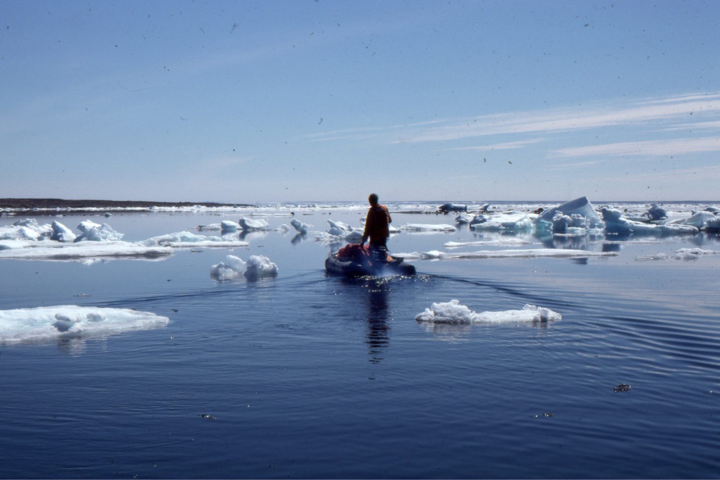
From 2 million years to 2 billion years: It’s now January 1976, confronted by a minus 25oC Ottawa, Canada, on my way to start a PhD at Carleton University. I’d never seen so much snow. My supervisor was to be Alan Donaldson, a Precambrian seds guru, who was pretty keen on me doing a thesis on the sedimentology and stratigraphy of a Paleoproterozoic succession on Belcher Islands, Hudson Bay. This collection of elongate, squiggly islands is held up by a 7-9 km thick, 1.8 to 2 billion year-old succession of stromatolitic platform carbonates, shallow marine siliciclastics, a banded iron formation, a turbidite succession, red beds, and two spectacular volcanic successions. When I asked Al which formation I should work on he said “do the whole shebang“. Ok! A tough working environment but great exposure of fabulous rocks (lots of boat – Zodiac work over 0oC seawater and inclement weather – my assistant and I wore life jackets so that, we were told, they could find our bodies for insurance purposes). Al was a great supervisor.
So over two 10-week field seasons (1976-77) I measured 20,000 m of section, 2000 paleocurrent directions, and a slew of petrographic analyses. I defended in June 1979.
Next stop Calgary for a two-year stint with Gulf Canada Resources, then in 1981 landed a job with the Geological Survey of Canada. In the GSC Calgary office most of that work was centred on field mapping and stratigraphy-sedimentology of Upper Cretaceous – Paleogene clastic sediments on Ellesmere and Axel Heiberg islands – mostly shallow marine, fluvial and delta settings. There were other bits and pieces in the Alberta Front Ranges, Yukon, and Mackenzie River. A move to the GSC Vancouver office in 1989 saw the emphasis change to Mesozoic sedimentology of one of the largest Intermontane basins in British Columbia, Bowser Basin, a foredeep with sediment derived from an obducted slice of oceanic crust.
Between 1992 and 1993 I realized I needed a change in Earth Science emphasis, and a logical choice was hydrogeology where I could use my knowledge of sedimentary rocks (sediment body geometry, composition, porosity-permeability and so on) and geological mapping to characterize fluid flow at both a basin-scale, and near-surface groundwater aquifer scale.
This culminated in a 4-year GSC pilot project to map and characterize aquifers in the greater Vancouver – Fraser Valley – Delta region of southern British Columbia, coordinating the expertise of colleagues with the use of shallow reflection seismic, ground penetrating radar, electromagnetics, gravity, MODFLOW modelling, and GIS data management of water-well databases and subsurface aquifer maps. Inserted between these programs was a brief secondment to the Hungarian Geological Survey in 1992 to help develop their basin analysis projects.
I quit the GSC in 1997 and moved with my Canadian family back to Aotearoa – New Zealand to work a 4-year teaching stint at University of Waikato, working primarily on Late Miocene – Pliocene siliciclastics and cool-water carbonates in Whanganui Basin (west North Island). From there a part-time position at Auckland University, teaching post-graduate basin analysis and undergraduate hydrogeology, and supervising (mostly) groundwater-related theses. But this position also required a significant weekly commute, and with an evolving disenchantment of academia I decided to form my own consulting company in 2005 – a company of one – and never looked back!
As a consultant I worked lots of NZ coal and oil-gas well-site geology (yes, I know…!), geothermal hydrogeology (Taupo region), basin-scale CO2 sequestration evaluation (with GNS), lithium-bearing brines in the Chilean Altiplano (base camp at 4000 m – the geology here is amazing), and a bunch of smaller jobs mostly groundwater-related. I loved this stage of my life – I was my own boss!
Now I am retired, tending to our organic kiwifruit orchard – we’ve been at it 25 years (all fruit exported so keep an eye open for it on your supermarket shelves), and maintaining the geoscience website that you must have linked to because you are reading this.
So, almost 50 years as a geologist. Time during 40 of those years was also spent as Editor and Associate Editor, mostly for the Canadian Society of Petroleum Geology and the SEPM including 8 years on the SEPM Council, and reviewer for dozens of journal papers. I still get requests for paper reviews, but I politely decline, noting that it is someone else’s turn.
Would I do it all again? Damned right, although I would probably try to insert a chapter on planetary geology into that life.
Henry Darcy’s pivotal experiments with sand-filled tubes (in 1856) established an empirical relationship between hydraulic gradient (that is basically an expression of the hydraulic potential energy available for flow) and discharge. A modern rewrite of the basic equation that he deduced from experiments, the eponymous Darcy’s Law, is:
Q = -KA(Δh/D) where (1)
Q is discharge (that has dimensions L3/T),
K is a proportionality constant, subsequently called the hydraulic conductivity (L/T)
A the cross-section area of a flow tube (L2) (Q is also proportional to A), and
Δh/D the head difference between two locations along a flow path, at distance D. Note that hydraulic head h is the sum of the pressure head and elevation head.
The hydraulic conductivity (a term borrowed from electrical theory), has dimensional units of distance and time (commonly expressed as cm/s, feet/s). Thus, in mathematical terms, K is expressed as a velocity, also known as the Darcy velocity.
Darcy’s empirically derived law is pivotal to modern, quantitative hydrogeological modelling. The description of his experiments and derivation of the law were published in Note D, an appendix to a lengthy report on the Dijon Fountains (680 pages!): Les Fontaines Purlieus’ de la Ville de Dijon (The Public Fountains of the City of Dijon). While the appendix might seem like an afterthought, it was in fact the culmination of two decades of observation, testing, experimentation, and the creative ability to extend his ideas below the surface, literally and figuratively.
How did Darcy arrive at this point of discovery?
Henry Darcy (1803-1858) was a French engineer who rose to prominence in the 1830s, at least in the public’s eyes, as the designer and executor of a modern water supply system for the city of Dijon, completed about 1840. Several other European cities modelled their own water supply networks on his design. The primary water supply for the Dijon network was a well dug into a groundwater (artesian) spring; the pipe supply network extended 28km – all gravity fed.
Darcy was familiar with the hydraulic theory and practice of the time; the theory of hydraulics was well established but the general understanding of aquifer dynamics was limited. Some of the important ingredients that contributed to his thinking and intuition were:
Bernoulli’s (1738) mathematical expression for energy conservation during fluid flow; in other words, flow requires an energy gradient. Bernoulli’s equation can be written as:
V2/g + z + P/ρ.g = a constant known as hydraulic potential (2)
where V2/g is kinetic energy, z the elevation head, and P/ρ.g the pressure head. By ignoring the kinetic energy component, that is insignificant for most groundwater problems, the equation reduces to a statement where hydraulic potential is the sum of z + P/ρ.g. The value of this statement is that it allowed Darcy (and us) to tease apart the components of hydraulic head in real wells and experiments.
He had developed an expertise with the practical problem of pressure losses between the entry and exit points of pipes used to transport water; he surmised and calculated the effects of surface roughness on energy, and therefore pressure losses.
Another crucial discovery, based on his work with pipes, was that at very low flow rates in small-diameter pipes, the head loss (or head gradient) was proportional to flow rate, that he would later discover could be applied to aquifer flow.
He was familiar with the flow of water through natural and constructed sand filters that were used to clean river water and was aware that frictional energy losses also applied to this kind of flow.
He had measured well drawdown for various pumping rates and observed well recovery.
He had general knowledge of aquifer geology and aquifer recharge by precipitation.
Darcy’s conceptual leap was to equate the physical nature of these observations (in pipes, filters, and the behaviour of boreholes) with flow through porous aquifer media. The experiments he designed and performed bridged the gap between concept and empirical evidence.
Darcy’s experiments
Darcy began his experiments in 1855. They were based in part on his observations of flow through sand filters, but what he needed was a way to quantify head loss (hydraulic gradient).
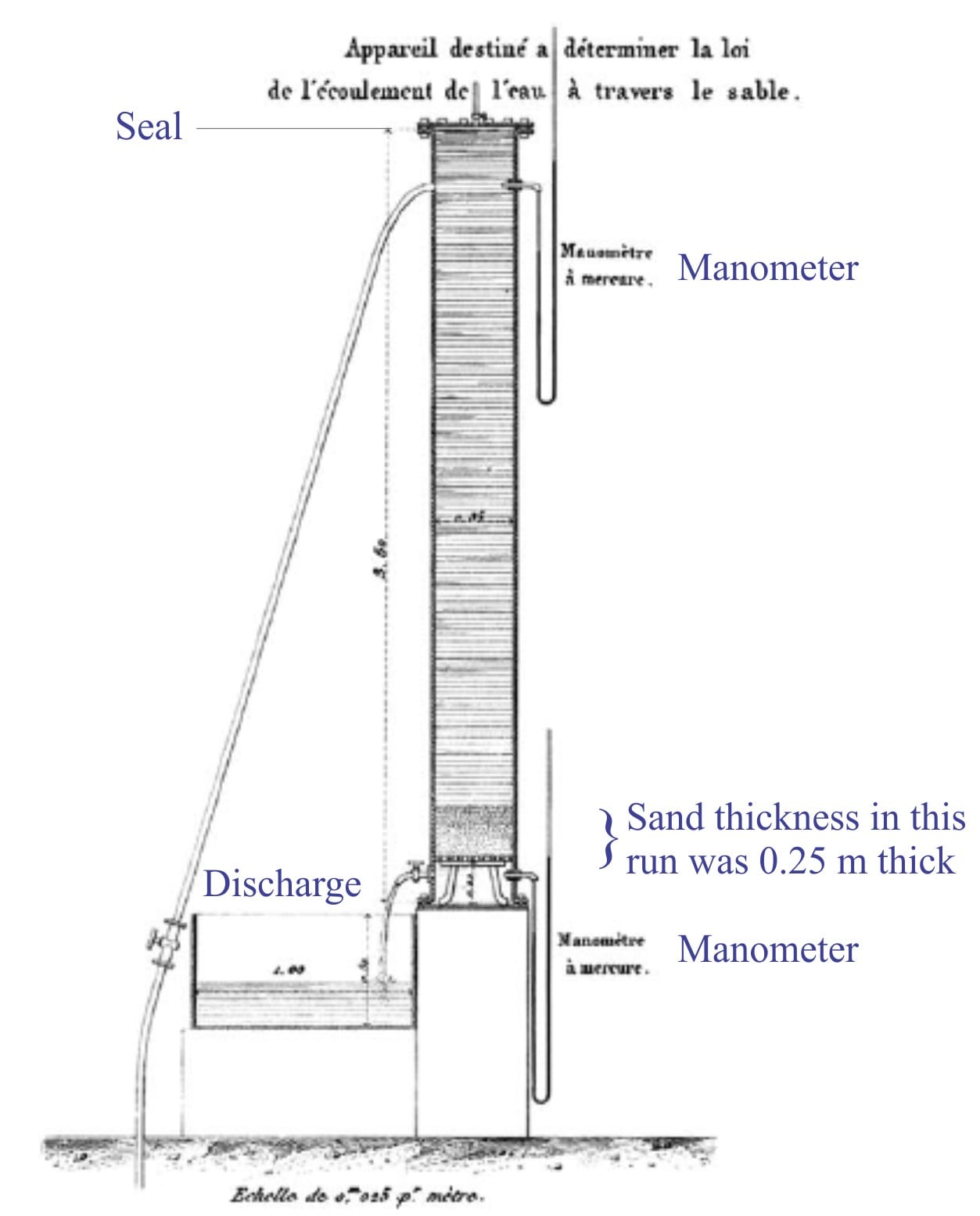
A diagram showing the original experimental apparatus is reproduced here. Modern groundwater texts commonly redraw the apparatus configuration to be more reflective of aquifer flow – I have added a duplicate diagram.
Darcy’s apparatus for determining the relationship between aquifer discharge and head loss, 1856. Figure 3 Plate 24, with some additional annotation
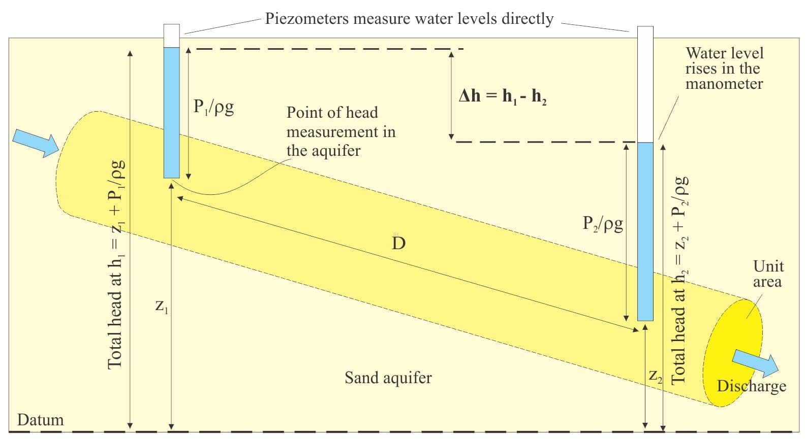
An alternative representation of Darcy’s experiment, shown as tube (pipe) flow in a sand aquifer. Instead of mercury manometers, the piezometers measure the water levels directly, relative to a datum. Each water level represents the total hydraulic head at the point of measurement in the aquifer. The distance D between piezometers allows the calculation of hydraulic gradient.
Darcy’s aquifer was represented by a vertical steel tube, sealed at both ends, with an air-bleed valve at the top. Two mercury manometers were used to measure pressures so that head values top and bottom of the tube could be calculated – the manometers measured atmospheric pressure ± the height of water. Water was added at the top of the tube and discharged from the base.
Darcy and his assistant performed several experimental runs. The tube was filled with water for each run. Sand was added from the top and allowed to settle on the bottom. The thickness of sand was varied systematically (this is D in the above expression), and for each sand thickness the flow rates were also varied. Flow of water into the tube was kept constant for each run; the discharge measured as volume per unit time (the vagaries of water supply at the time meant that keeping flow constant was a bit of a problem). Once steady state conditions had been established in each run, the manometer (pressure) levels were read.
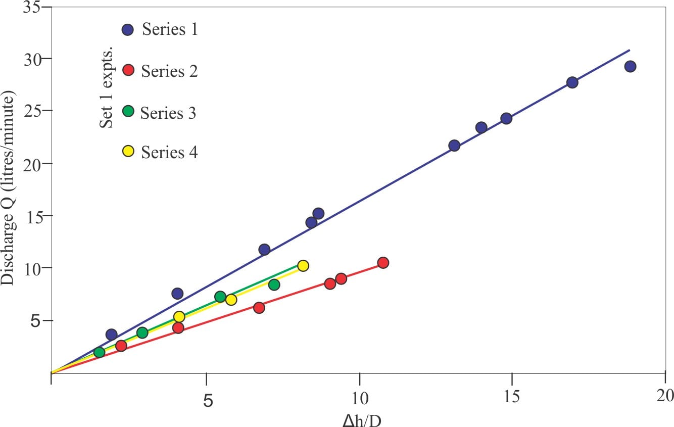
The following graph shows the observed linear relationship between discharge Q and head loss (or head difference) based on Darcy’s data.
Darcy’s data for Set 1 experiments (there were two sets), replotted as Q versus head gradient for each thickness of sand. Modified from Brown, 2002, Fig. 6.
Darcy’s key observations were:
Discharge is proportional to the head loss, or head difference along the flow path (Q ∝ Δh), and
Discharge is inversely proportional to the distance that water travels between the two points of head measurement (Q ∝ 1/D) (in his experiments this is the thickness of sand).
He expressed the proportionalities as: Q = KA (h1 + z1) – (h2 + z2)/D (3)
where Q, K, A, and D as noted above, h is the pressure head, z is the elevation head at the two points of measurement (1 and 2) that are a distance D apart. This is Darcy’s Law. The form of the equation is basically the same as equation (1).
He noted that K varied depending on the sand used (particularly its packing that probably varied slightly for each experiment). We now know that K (hydraulic conductivity) not only varies with differences in the porous medium, but also with the nature of the liquid. Thus, if the sand is the same in two separate experiments, but water is used in one and oil in the other, then the values of K will be different. Later considerations by other workers would establish that K is also a function of dynamic viscosity.
And so…
Darcy’s Law tells us that, under steady state conditions, there must be a hydraulic (head) gradient for flow to occur in an aquifer; in essence it restates the fundamental physical principle that for mechanical work to be done (i.e., to move water from one location to another) there must be an energy potential.
The Law also provides a quantitative solution to determining the parameters for groundwater flow, provided we know something about the porous medium and the fluid itself (that is expressed as hydraulic conductivity). Of course, we can also determine K if we know Q and Δh, and we can measure K experimentally using a permeameter – an instrument that looks similar to Darcy’s original apparatus.
Darcy’s Law describes a flux, and as such is cast in the same mathematical form as Ohm’s Law (current is proportional to voltage), and Fick’s Law (molecular diffusion is proportional to a concentration gradient.
Darcy’s Law is a crucial component of fluid flow modelling, particularly for solving important questions about groundwater, for example the sustainability of aquifers to pumping.
Credits: The historical background to Darcy’s life, his scientific and social contributions were gleaned from Freeze (1994; Brown (2002- open access); and Simmons (2008 – PDF).
The title page to Johann Lehmann’s 1756 publication on stratigraphy
Preamble: This post outlines the development of formal stratigraphy, focusing on Chronostratigraphy. Entire books have been devoted to this topic; one of the most entertaining and enlightening is Martin Rudwick’s excellent account of the conduct of 19th century gentlemen who argued the case for the Devonian. My account is woefully brief, but there you have it…
This is part of the How To…series on Stratigraphy and Sequence Stratigraphy
The role of a stratigrapher is to decipher the organisation and origin of strata, and the order of events recorded therein. Stratigraphy is all about space and time.
The idea that strata might be ordered in a predictable manner dates back centuries. Imagine an 18th century surveyor or land-man wandering the hills in search of coal, and observing seams that were associated with sandstone, mudstone and limestone, and that the arrangement of these strata was the same from one locality to another. Finding a particular limestone might lead the surveyor to predict the presence of coal seams, if not at the surface, then beneath it.
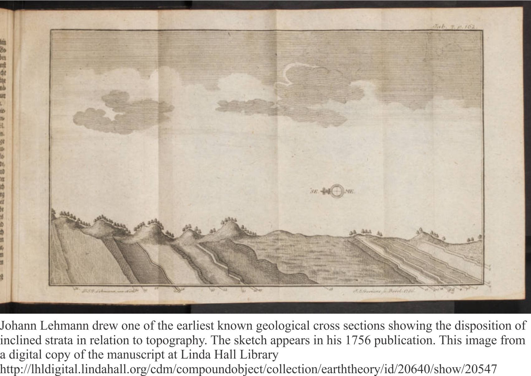
One of the earliest attempts at formal stratigraphic classification was Johann Lehmann’s three-fold subdivision of rocks, published in 1756. His scheme combined a description of strata, placing them in order, oldest at the bottom:
Primitive, or Primary crystalline rocks, lacking fossils.
Secondary stratified, fossiliferous rocks (some derived from the Primitives), and
Surficial, unconsolidated alluvium and colluvium.
The concept of relative time encapsulated by this succession was based on Steno’s axioms. Towards the end of the 18th century, the influential German geologist Abraham Werner expanded Lehmann’s classification, claiming it to be global in extent, to include a Primitive (crystalline) Series, a Transitional Series (greywackes, limestones), a Stratified, or Secondary Series (much like Lehmann’s), an Alluvial Series to which the term Tertiary was applied by some, and a Volcanic Series. Like Lehmann, Werner’s scheme also combined the physical attributes of rocks and their relative age. Werner is also remembered for advocating that all rocks had precipitated at different times from a universal ocean – a concept that came to be known as Neptunism.
Throughout late 18th and 19th centuries, the naming of rock units became widespread in Europe, Britain, and North America, usually beginning with local knowledge of commonly occurring successions that were traced and mapped farther afield. Fossils became an important part of this development, where it was recognized that certain taxa and assemblages of fossils were characteristic of particular stratigraphic intervals. In England, this was exemplified by William Smith’s iconic map. Assemblages of rocks having identifiable lithological and fossil characteristics were given names that are still in use today; the progress of mapping demonstrated the repetition of characteristic successions, or Groups of strata. Thus, Old Red Sandstone was overlain by Mountain Limestone followed by Coal Measures; the group was subsequently called the Carboniferous Order by Conybeare and Phillips in 1822 (Phillips, 1837), and later the Carboniferous System.
The first half of the 19th century saw a proliferation of Systems, each containing characteristic rocks and fossils, where the relative time relationships of fossils are strategic. In England, and no doubt elsewhere, there were competing views on the placement of system boundaries, and whether systems once established, could be split – some of these rivalries became bitter, even publicly so (Rudwick, 1985). For example, the Carboniferous was eventually divided into Devonian (based on the succession in Devon) followed by Carboniferous, the Cambrian was inserted between Primary rocks and the Silurian (by Roderick Murchison), and later the Ordovician (Charles Lapworth) between these two Systems.
It is important to remember that prior to Charles Darwin (1859) and Alfred Wallace, there was no accepted scientific theory that explained the transition from one species to another – the observation that species change through successive strata does not require a biological mechanism – just a good pair of eyes. Of course, post-Darwin and Wallace, the underlying theoretical mindset changed.
By the late 19th century all major system names, as we know them, had been proposed:
Sedgwick – Cambrian, 1835
Lapworth – Ordovician, 1879
Murchison – Silurian, 1835
Murchison & Sedgwick – Devonian, 1839
Conybeare & Phillips – Carboniferous, 1822
Murchison – Permian, 1841
Von Alberti – Triassic, 1834
Von Humboldt – Jurassic, 1799
D’Halloy – Cretaceous, 1841
Aduino – Tertiary, 1760
Denoyers – Quaternary, 1829
Charles Lyell (1833) created a similar scheme for Tertiary strata, giving us Pliocene, Miocene and Eocene, based on the more modern appearance of fossils; characteristics that clearly set them apart from all Secondary strata. Based on the distinctiveness of fossils in each of Werner’s Transitional, Secondary, and Tertiary Series, Lyell coined the now familiar terms:
Cainozoic (Tertiary) fossils have modern affinities, mammals, and the appearance of Homo sapiens,
Mesozoic (Secondary) the proliferation of ammonites and dinosaurs,
Paleozoic (Transitional) ancient life forms: first invertebrates, first fish, first plants,
Azoic (Primitive)
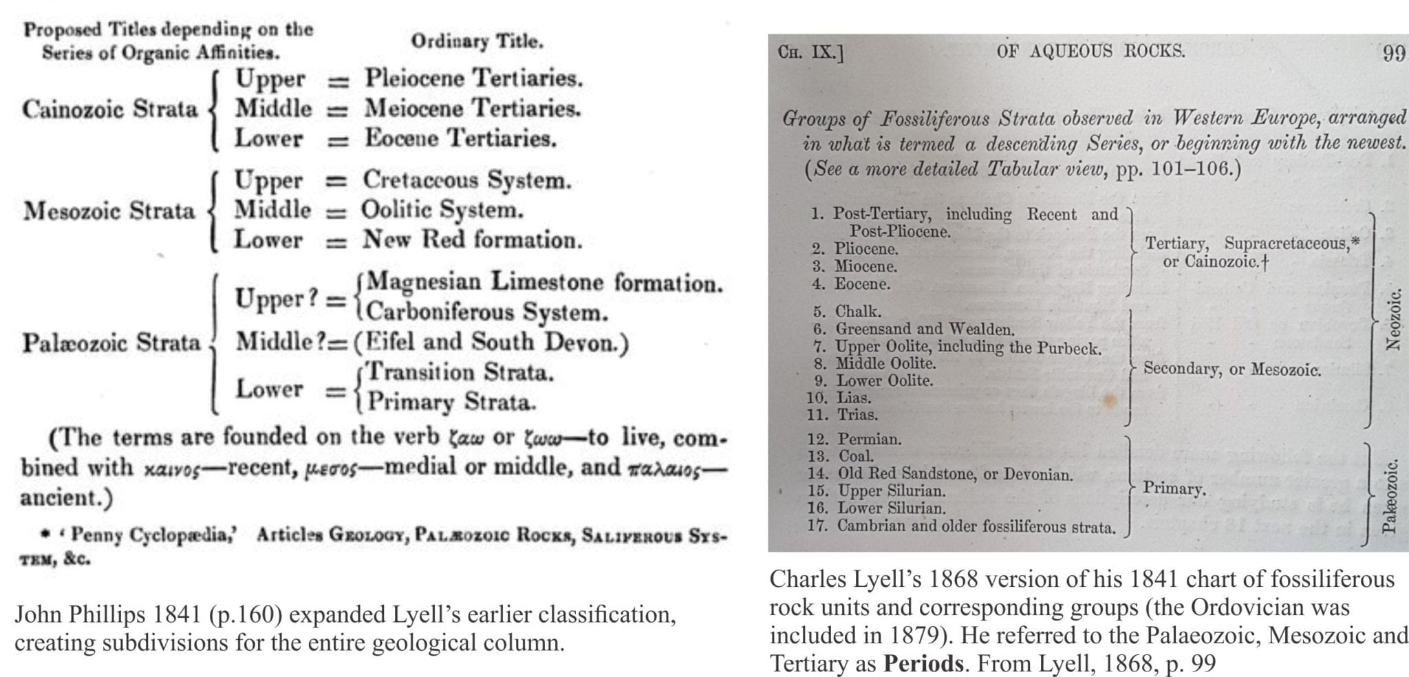
Publications by John Phillip and Charles Lyell in 1841 extended the system of classification to the entire geological column. Phillips used Lyell’s earlier divisions and subdivided them into Lower, Middle and Upper. Lyell went one further, and referred to the Primary, Palaeozoic, and Tertiary as Periods, acknowledging their chronostratigraphic significance.
Development of a more formal system of Eras and Systems as fundamental units of geological (relative) time was based entirely on fossils. An early proponent of this strategy was James Dana who in 1880 referred to the Cenozoic (Cainozoic), Mesozoic, Paleozoic and Archean as Times, each Time consisting of Eras (Devonian etc.), divisions within each Era such as Early, Middle and Late were called Periods, and subdivision of Periods into Epochs. To complete the duality of the Geological Time Scale, Dana applied the corresponding terms Series, Systems, Groups and Stages respectively to the equivalent rock units (Dana, 1894). Dana’s time scale has a particularly modern look to it.
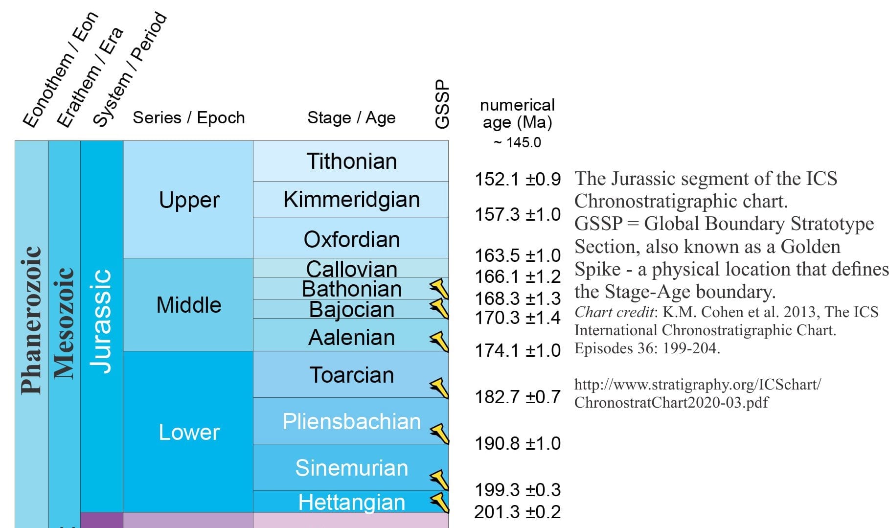
Dana’s Geological Time Scale, and those of other geologists, have in the intervening 140 years, gone through many iterations, modifications, additions and subtractions. One of the most important contributions was the addition of radiometrically determined ages, that changed the relative time scale based on fossils and superposition, to a numerical scale. Geologists could now talk of events 200 million years ago (200 Ma) in addition to referring to Early or Lower Jurassic.
In 1974 the International Commission on Stratigraphy was established, with the aim of standardizing system boundaries. The modern Time Scale moved Dana’s time units to the left – the Devonian is now a Period/System, and the corresponding Era (time) is the Paleozoic. There is now reasonable international consensus on the format and content of the Geological Time Scale. However, the entire enterprise is continually under review; witness the debate on the Anthropocene, the geologically youngest, human-influenced epoch.
We now employ three primary components in formal stratigraphy:
Time units (Era, Period) that refer only to geological time and not process.
Time-rock units; strata deposited during a specific interval of time (System, Epoch).
Rock Units that refer only to the composition and mappability of strata (Formations, Groups).
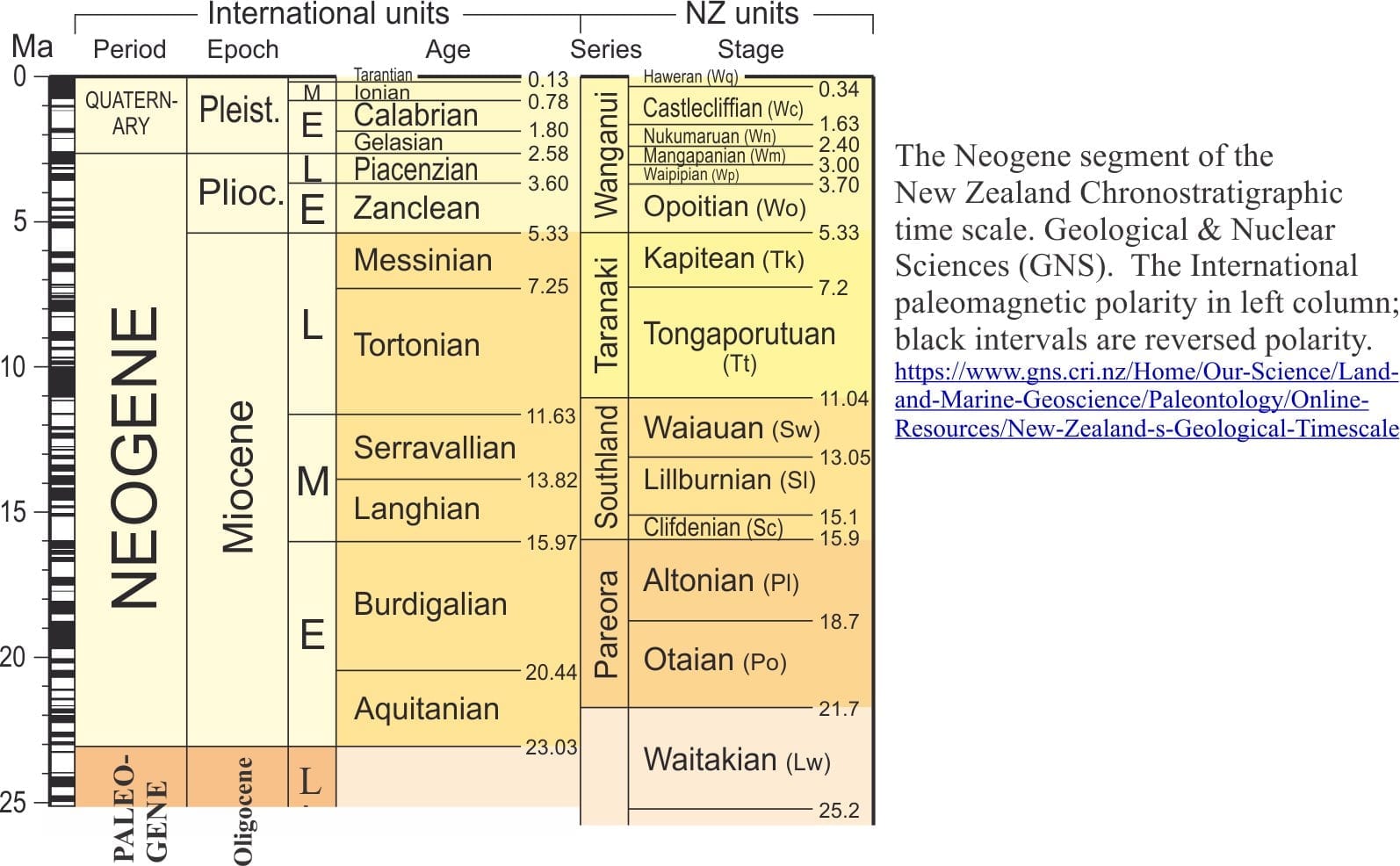
The International Chronostratigraphic time scale provides the framework for more local stratigraphic schemes. For example, much of the New Zealand Cenozoic time scale is based on marine faunas that have little correspondence with northern Hemisphere taxa. Therefore, the New Zealand scheme has Series and Stages, superimposed on International Ages and Epochs.
Formal stratigraphic schemes
Lithostratigraphy
Formal lithostratigraphy is concerned with the description and mappability of rocks, using physical, fossil, and mineralogical attributes. The basic lithostratigraphic unit is the Formation. A Formation must be mappable; it must have well defined and easily identifiable surface or subsurface contacts. Contacts can be abrupt or gradational; they may be unconformable, but an unconformity should not pass through a formation. There is no reference to time. Formations can be subdivided into Members or smaller entities like Beds. Two or more Formations can be named as a Group.
The boundaries of Formations are invariably diachronous. The definition does not include any interpretive quality. Formations require Type Sections, that are locations or outcrops that contain most of the unit’s defining characteristics. Type Sections should be accessible.
Formations need not consist of a single lithology; interbedding of two or more lithologies is common. What is important is the internal consistency of the interbedded nature of strata compared with underlying or overlying formations. The geometry of lithostratigraphic units is also highly variable: sheets, lenses, shoestring, splits, and pinch-outs.
Chronostratigraphy
Prior to the advent of radiometric dating (early 20th century), the concept of geological time was based on superposition and the observed transitions from one taxon to another (fossils); this was relative time, where stratum A is older than overlying stratum B. While the immensity of time was in little doubt (at least among the 19th century scientific community), there was no way to quantify it in terms of years. Intelligent estimates were made based on biblical genealogy (Ussher, Kepler), the rate of Earth surface processes (Lyell, Darwin), and the rate of Earth cooling (Comte de Buffon, Lord Kelvin).
One of the first attempts to radiometrically date rocks (using isotopes of uranium) was made by B. Boltwood in 1907, a Yale University professor. Since then the science and technology of radiometric dating has advanced to the point where minute zones in a single zircon crystal can be dated.
The evolution of chronostratigraphic time scales is noted above. Radiometric dating has provided dates for all the important time and time-rock subdivisions.
Biostratigraphy
The chronological ordering of strata is based on two principles: superposition and the observed stratigraphic variations in fossils and fossil assemblages. These principles provide the foundations for the stratigraphic time scales we use today. The principle of faunal succession is based primarily on the appearance of specific organisms in certain strata that, in progressively younger rocks (deemed younger because they occur higher in the stratal succession), morph into different, but related organisms.
An early attempt to systematically apply variations in species was published by Albert Oppel (1856-1858), who described successive changes in ammonites, beginning with the lowest and oldest Psiloceras Planorbis. He proposed 14 Zones within the Lower Jurassic Lias of England and Germany. Oppel observed that the range of various species was variable; some had narrow stratigraphic ranges, others ranged over greater thicknesses of strata. However, all could be regarded as temporary. He defined a zone by the first appearance of a species, the overlying zone by the appearance of a new species and so on. Any species may range through more than one zone, but its first appearance was considered unique. The concept of zone, or biozone forms the basis of modern biostratigraphy.
Biozones (zones) are the fundamental biostratigraphic units. The five formal biozones are: range zones, interval zones, assemblage zones, abundance zones, and lineage zones. Each biozone is distinct. The International Stratigraphic Commission, and the North American Stratigraphic Code provide complete definitions and rules for their usage.
Magnetostratigraphy
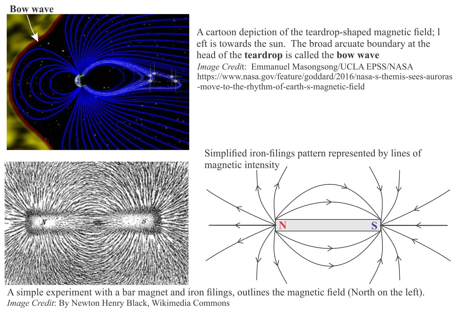
Earth’s magnetic field is generated by a hot (4000-5000oC), fluid-like, iron-nickel rich outer core that moves slowly around a solid iron inner core. The shape of the magnetic field is approximated in a simple experiment using a bar magnet and iron filings. The magnetic field is vertical at the poles and horizontal at the equator. Between the magnet poles, the iron filings approximate lines of equal magnetic intensity. In a three-dimensional Earth, we know that magnetic North moves in a circuitous path around the Geographic North Pole (in fact it has moved more than 1000 km since 1831 when first measured by James Ross). We need two measurable parameters to define the orientation of the magnetic field at any point on Earth’s surface:
The angle between magnetic north and Geographic north – the declination, and
Inclination (or magnetic dip), the up or down angle of the field measured from a horizontal plane at any point on the surface. This is approximated by a compass needle pointing down in the northern hemisphere (positive dip), and upwards in the southern hemisphere (most commercial compasses don’t show this because they have been balanced).
A couple of early 20th Century geophysicists, Bernard Brunhes and Motonori Matuyama, devised experiments where remnant magnetism was measured in volcanic rocks. The rationale is that when lavas solidify, iron-bearing minerals in the rock, especially basalt, will act like tiny fossil magnets that record the direction (polarity) of the magnetic field at that time. Their experiments demonstrated that the magnetic field had indeed reversed in the distant past. If the age of the rock being measured is known, then so too is the age of the reversed magnetism, a method now extended to sedimentary and other kinds of volcanic rock. It has since been established that reversal of Earth’s magnetic field has occurred every 200,000 to 300,000 years over the last few million years. The last reversal took place 780,000 years ago; this is called the Brunhes-Matuyama Reversal.
The formal stratigraphic measure is the magnetostratigraphic polarity unit. The unit is recorded as Normal Polarity (north pointing) or Reversed Polarity for a body of rock. According to the International Commission on Stratigraphy, a polarity unit is:
a single polarity of magnetization;
an intricate alternation of normal and reversed polarity of magnetization;
having dominantly either normal or reversed polarity, but with minor intervals of the opposite polarity.
An example is shown on the New Zealand stratigraphic chart above.
J.D. Dana, 1894. Manual of Geology: Treating of the Principles of the Science with Special Reference to American Geological History. 4th Edition. American Book Company, 1088 p.
J. Lehmann, 1756. Versuch einer Geschichte von Flötz-Gebürgen (Attempt at a History of Stratified Mountains). Berlin. Available to read at Linda Hall Library
Lyell, 1833. Principles of Geology. John Murray, London.
Lyell, 1868. Elements of Geology, or the ancient changes of the Earth and its inhabitants as illustrated by geological monuments. Appleton and Company. 803p.
A. Oppel, 1856-1858. Die Juraformation, Englands Frankreichs und des Sudwestlichen Deutschlands. The manuscript is available, in German
J. Phillips, 1837, Treatise on Geology. Longman, Orme, Brown, Longman, London. The text can be read in digital form on Internet Archive
J. Phillips, 1841. Figures and descriptions of the Palaeozoic fossils of Cornwall, Devon and west Sommerset.Longman, Brown, Green, and Longmans, London. Digital version available
M.J.S. Rudwick, 1985. The Great Devonian Controversy: The shaping of scientific knowledge among gentlemanly specialists. The University of Chicago Press, 494 p.
H.S. Williams, 1893. The making of the Geological time scale. Journal of Geology, v. 1, p. 180-197.
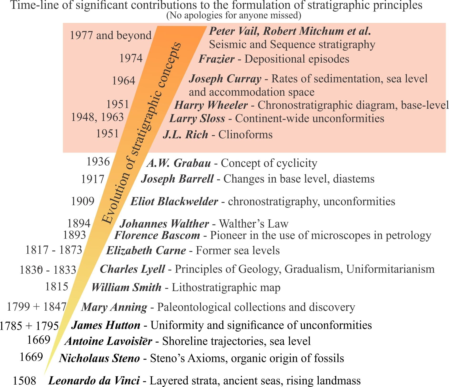
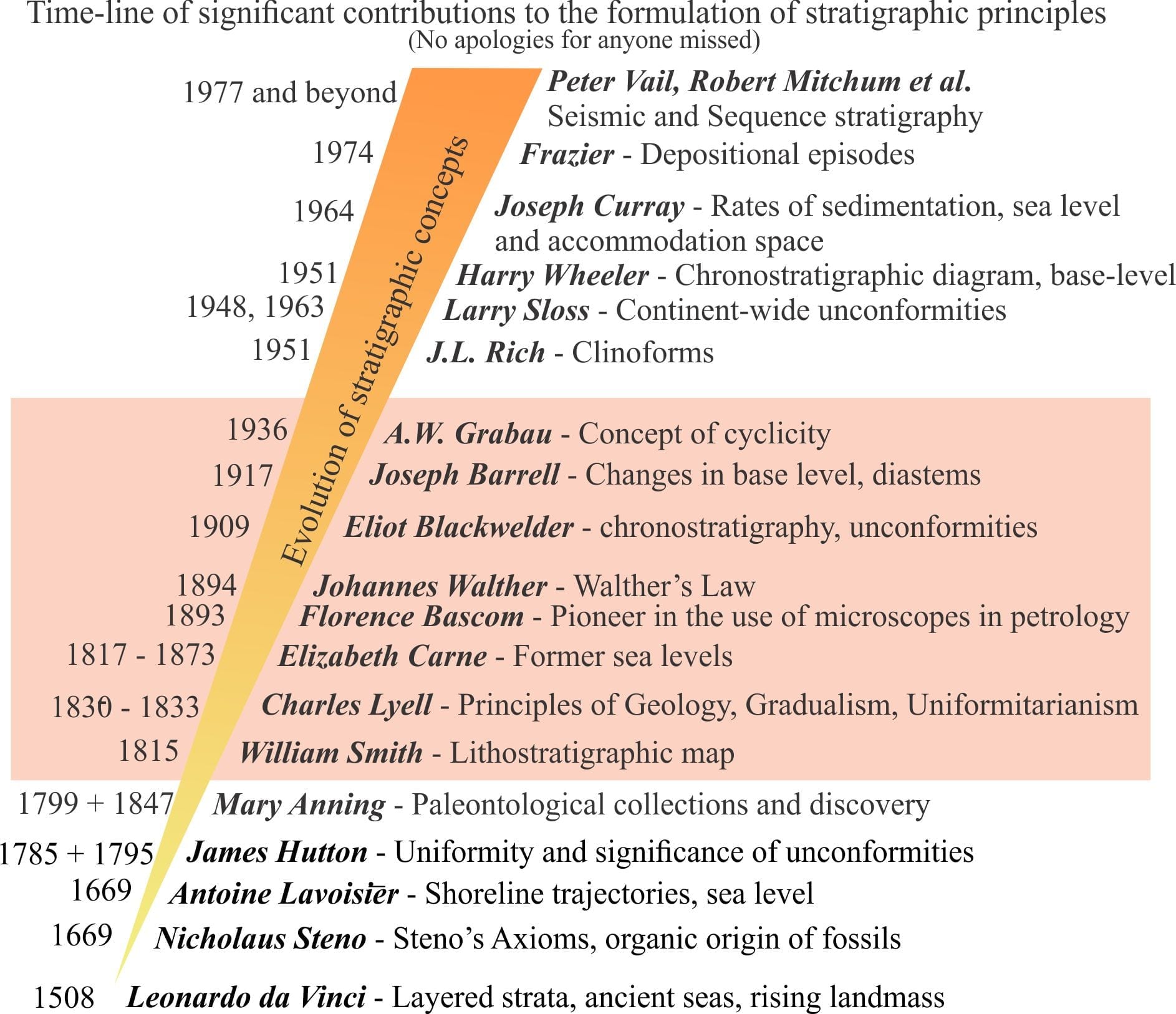
This is the third of three posts that look briefly at the development of stratigraphic concepts and the people responsible for them, spanning 1950 to 1977. This period witnessed the maturing of modern stratigraphic concepts from formal, descriptive lithostratigraphy to less formal genetic stratigraphy that was more concerned with depositional processes and time, particularly the recognition of chronostratigraphic surfaces.
This is part of the How To…series on Stratigraphy and Sequence Stratigraphy
Preamble: My intent was to write a single post on this topic, as an introduction to Stratigraphy in general, and Sequence Stratigraphy in particular. But I kept adding names to the timeline, and got carried away with some of the characters on it. So the number of posts was expanded.
John Rich (1884-1956)
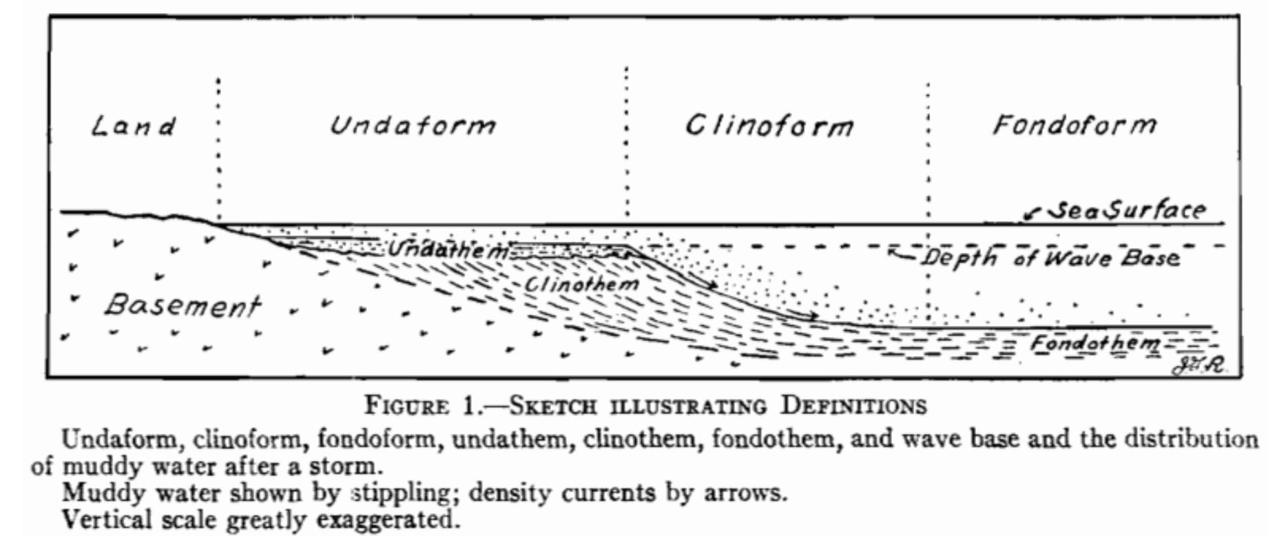
John Rich was another all rounder, publishing widely on sedimentology and stratigraphy, with excursions into submarine canyons and shelf to basin facies transitions. It was his examination of the latter, combined with ocean floor geomorphology, that led him to propose the concept of clinoforms, geometric components that are a critical element of modern sequence stratigraphy. He defined a clinoform as a sinusoidal surface extending across the shelf from wave base to the base if the adjacent slope. Shoreward of wave base is the undaform; beyond the base of slope is the fondoform. (Rich, 1951) Together they represent a time, or chronostratigraphic surface. Based on modern analogues of shelf, slope and deep basin, he identified prominent sedimentary facies and depositional processes that could be used to identify and interpret similar arrangements in the rock record.
John Rich’s illustration of undaforms, clinoforms, and fondoforms. He was one of the first to use wave-base as an important boundary
The terms undaform and fondoform have all but faded into obscurity; these days, all are generally referred to as clinoforms, and their stratigraphic representation as clinothems. The term clinoform is no longer restricted to shelf-slope morphologies, and can be used at almost any scale (Patruno, W. Helland-Hansen, 2018). For example, topset, foreset and bottomset beds of fan deltas are typically bound by clinoforms.
Rich’s use of wave base is also important; it is the depth limit at which waves and wave orbitals cease to move sediment across the sea floor. It represents a significant boundary between inshore and deeper shelf sedimentation; we now use it to define the outer limit of the shoreface. He surmised that during sea level fall, undaform sands, particularly those across a beach, would move seawards in concert with wave base, a process that might continue to the shelf margin – we can almost hear him thinking shelf margin, or forced regressive sand clinoforms.
Larry Sloss (1913-1996)
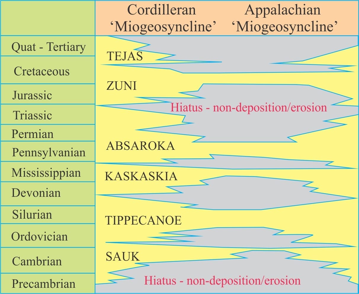
Sloss, Krumbein and Dapples first published this diagram in 1949. It expands Blackwelder’s ideas on unconformity bound sequences
When Larry Sloss joined the faculty at Northwestern University in 1947, he became part of a geological powerhouse triumvirate with Edward Dapples and William Krumbein. It was here that Sloss’ ideas on rock assemblages and unconformities came to fruition, being impressed with Blackwelder’s earlier descriptions of unconformity-bound successions, and in 1949 he, with Krumbein and Dapples, first presented a stratigraphic framework that incorporated lithostratigraphic successions, or sequences, bound by unconformities. Part of their rationale was to provide a stratigraphic framework within which they could map sedimentary facies. The concept was applied to rock assemblages they had traced across continental USA. The audience of the day was skeptical, but the concept and the names they gave to each sequence are still used today (Sloss et al. 1963). They recognised that the amount of time missing at each unconformity varied fairly systematically from the western Cordillera to the Appalachians. The 6 sequences incorporate strata from late Precambrian to the present, each representing 10s of millions of years. For example, the time value of the Absaroka is about 117 million years.
Harry Wheeler (1907-1987)
Sloss et al. (1949) provided one of the first definitions of sequence as a stratigraphic entity, but restricted it to “assemblages of formations and groups … without specific time significance…” (quote from Pemberton et al. 2016). Harry Wheeler thought otherwise, and produced a definition that completely negated all lithostratigraphic connotations: his sequences contained assemblages of strata bound above and below by unconformities, that were independent of formal lithostratigraphic units (Wheeler, 1958) – a definition that basically pre-empted by 20 years, the foundations of sequence stratigraphy. This view of the stratigraphic world bordered on heresy to 1950s through 70s stratigraphers, for whom formations were the cornerstone of objective geological enquiry. Formations are based on composition and mappability; formation boundaries are essentially diachronous. Wheeler argued for the complete opposite. His proposal was one of the most important of the modern era, but was ignored for many years.
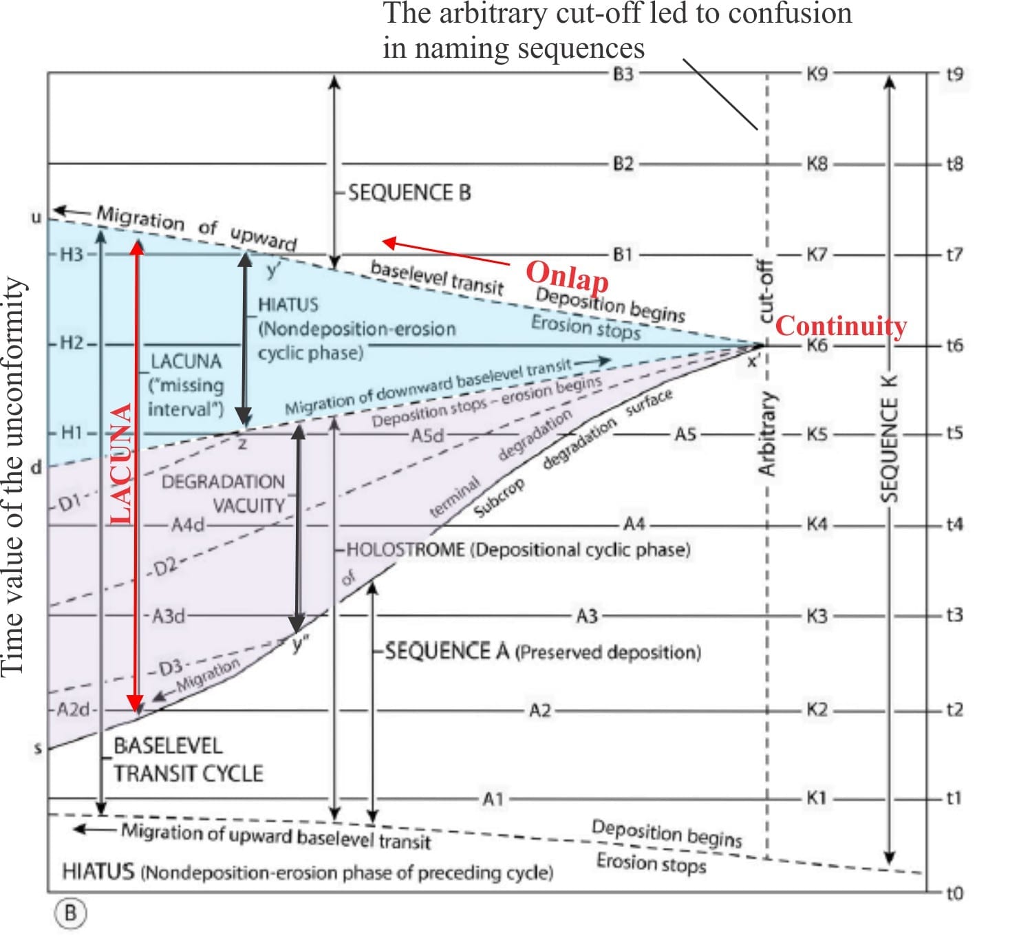
Wheeler’s published his classic chronostratigraphic representation of unconformities in 1964, where he defines lacuna, hiatus, and degradational vacuity. Compare this diagram with his Figure 2b. Annotation in red has been added.
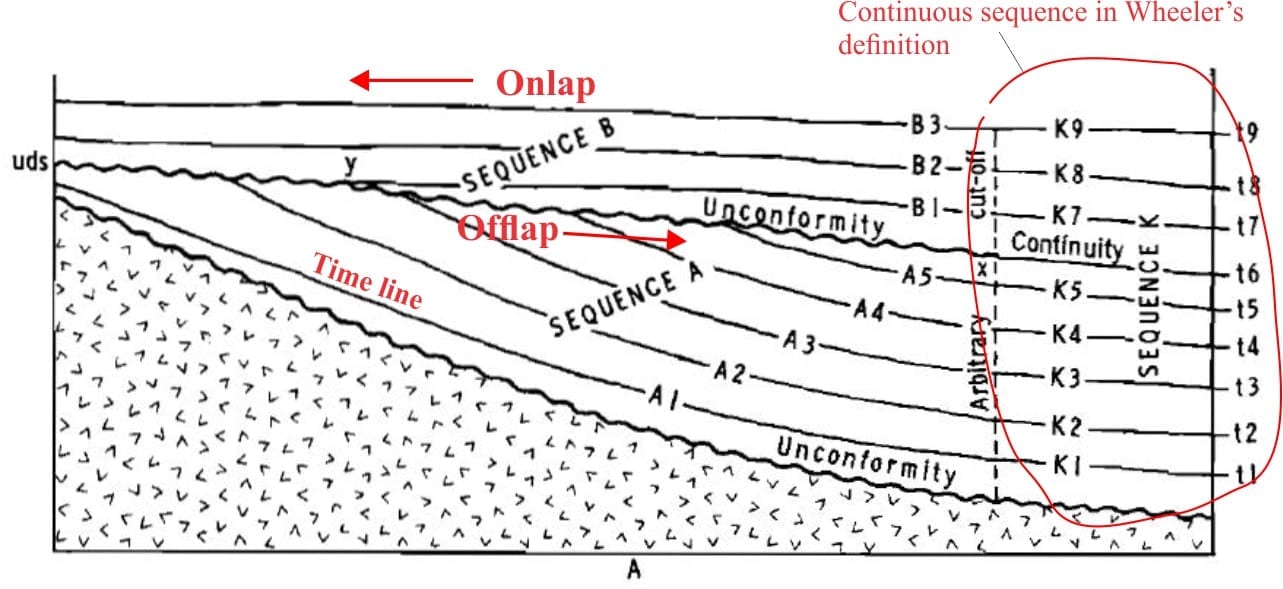
His explanation of sequences is best delivered by a figure published in 1964 where he introduces his own chronostratigraphic language. The Wheeler Diagram is a time-stratigraphic representation of two sequences, A and B, separated by an unconformity on the left, and a continuity on the right (he did not use the more recent expression correlative conformity, but that is what he meant). Timelines are indicated for each sequence. With one exception (discussed below) Figure 2a would not look amiss in any modern discussion on sequence stratigraphy where Sequence A shows a pattern of offlap, and Sequence B onlap.
Wheeler’s Figure 2a shows the geometric relationships between sequences A and B, and the inferred timelines. Annotation in red has been added.
Figure 2b is a Time-Area (space) or chronostratigraphic plot of the stratigraphy in 2a. The Lacuna encompasses the total time missing at the unconformity, and is divided into an Hiatus (a term introduced by Grabau) which is a non-depositional or erosional episode above the unconformity, and an Erosional or Degradational vacuity below it (i.e. the time represented by rocks removed by erosion). Using Barrell’s terminology, he defined the line separating these two as the base-level transit that progresses from left to right (towards the continuity). The ‘onlap’ stage is defined by base-level transit to the left.
One important criticism of Wheeler’s scheme, in a sequence stratigraphic context, is the “arbitrary cut-off” between the unconformity and continuity (Bhattacharya and Abreu, 2016). For Wheeler, the cut-off separates a different sequence (sequence K in his Figure 2a). We now know that the assemblages below and above the continuity are an integral part of sequences A and B respectively.
Joseph R Curray
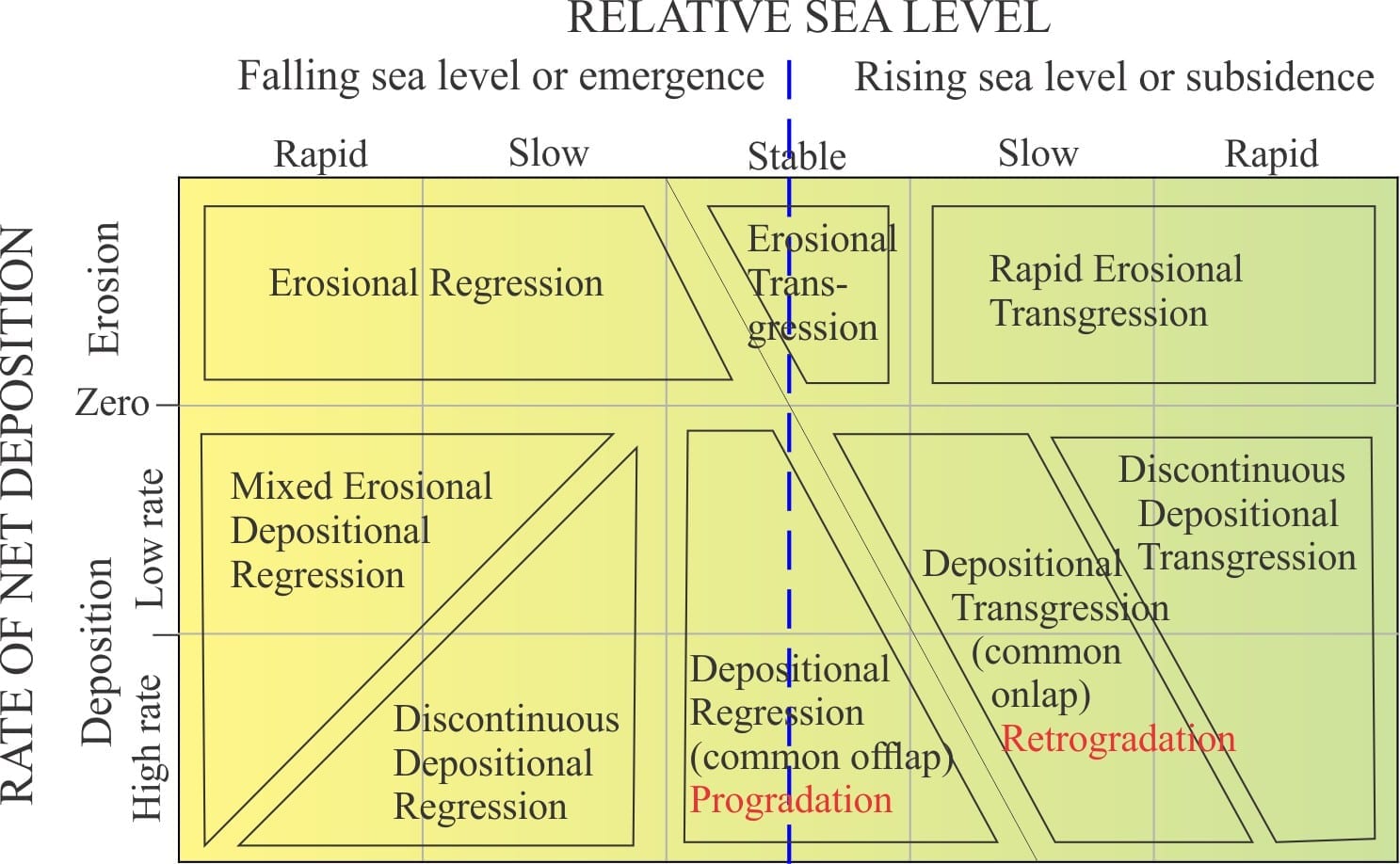
The 1960s were witness to burgeoning understanding of sedimentary facies, the dynamic controls on deposition, and changing sea levels (or base levels); in other words, a recognition that sediment deposition was a pretty complex process. In this context, Joseph Curray’s contributions centre on the processes of deposition versus non-deposition and erosion, as they relate to variable rates of sea level change (base level) and sedimentation. These ideas are nicely summarized in one of his diagrams, published in 1964.
Curray’s 1964 diagram shows partitioning of erosion or deposition, by comparing the interplay between the rate of deposition and the rate of sea level fluctuation.
The diagram partitions regions of deposition or erosion depending on the interplay between base level and sedimentation. Although he did not discuss explicitly the concept of sediment accommodation space (a concept that is central to modern sequence stratigraphy), it is implicit in the diagram. Curray used the term relative sea level because he recognised the varying roles of eustasy, basin subsidence, tectonics, and sediment supply, and net deposition because of the competing roles of erosion and sedimentation.
David Frazier
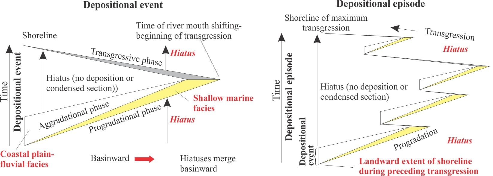
Frazier worked extensively on Gulf Coast Cenozoic stratigraphy, including modern and ancient deposition on Mississippi Delta. He recognized a fundamental relationship between periods of deposition alternating with hiatuses; he referred to these cyclic alternations as depositional episodes. Each episode contains a succession of facies that represent specific styles of deposition associated with fluctuating sea levels (Frazier, 1974).
Fraziers diagram shows the alternation of progradation-aggradation with periods of non-deposition (hiatuses) or development of condensed sections, that he defined as depositional episodes.
Each episode begins with progradation of coastal facies and/or delta lobes during sea level stillstand, and at the same time,
Aggradation of coastal plain and fluvial facies. The episode begins at the maximum landward extent of the shoreline from the preceding transgression. Aggradation decreases and progradation increases with time as sea level falls.
During the transgressive, or terminal phase, sediment supply is reduced, and estuaries migrate up the earlier-formed river channels on the coastal plain. Seaward, on the adjacent shelf or delta platform, deposition is limited to fine-grained pelagic and hemipelagic sediment resulting in thin, condensed stratigraphic sections, or in the case of no sediment supply, an hiatus.
Depositional episodes may be punctuated by smaller scale cycles of regression-transgression (these are events in the Frazier diagram), but the overall pattern of sea level change is stillstand, followed by sea level fall, and transgression (or retrogradation) – much like Barrell’s 3rd order cycles superimposed on longer period 2nd order cycles. Frazier also notes that the point of maximum transgression (and the end of the episode) corresponds to an hiatal surface that is synchronous across the platform and slope.
Peter Vail, Robert Mitchum et al.
Peter Vail and Robert Mitchum continued to expand the ideas of Sloss (no surprise there really), Frazier and others. Their names and those of their colleagues at Exxon are basically synonymous with modern Sequence Stratigraphy. The rapid expansion of reflection seismic data coupled with extensive international drilling (and the accompanying wireline logs that also were developing rapidly), plus a burgeoning microfossil database, created an opportunity to develop the Sloss-Blackwelder-Wheeler ideas into a stratigraphic model that emphasized time, key stratigraphicsurfaces such as unconformities, and depositional systems for which an understanding of depositional processes is key. AAPG Memoir 26 (1977) was devoted to papers on seismic stratigraphy and sequence stratigraphy by Vail and his Exxon colleagues.
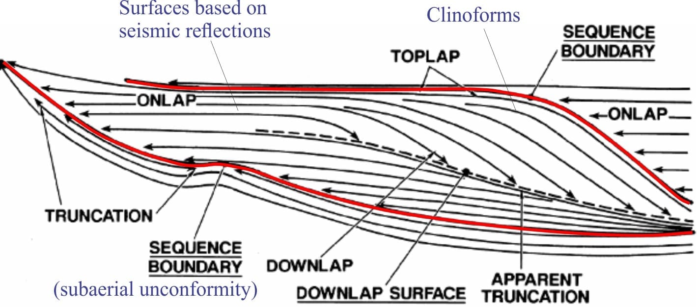
The impetus for this conceptual revolution was the rapidly improving methods of acquiring and processing reflection seismic, developments tied inextricably with the hydrocarbon exploration industry. Seismic profiles allowed the identification of packages of strata, their geometry, stacking patterns, and lateral extent. This is where clinoforms came into their own, wherein reflections are considered to approximate timelines. In their original definition, a sequence is bound by unconformities and correlative conformities (what Wheeler called continuities), where relatively conformable packages of strata are bound by lap out surfaces: onlap, toplap, and downlap. Sequence bounding surfaces delineate important events across a basin.
One of the early diagrams of Peter Vail and his Exxon colleagues, showing sequence boundaries, lapout boundaries, and clinoforms. that define a stratigraphic sequence
In their early analyses the Vail crew argued that eustasy was the primary driver of sea level fluctuations, and by correlating sequences they constructed a global sea level curve (note that the actual definition of sequences does not depend on this model). Not surprisingly this caused consternation in many quarters because our knowledge of sedimentary basin dynamics (subsidence profiles, tectonics, and the influence of sediment source area and climate) was also evolving rapidly. One outcome of the ensuing discussions, is that we generally refer to relative sea level, acknowledging that at any time it is the result of some combination of eustatic, subsidence and tectonic processes.
J.P. Bhattacharya and V. Abreu, 2016. Wheeler’s confusion and the seismic revolution: How geophysics saved stratigraphy. Sedimentary Record (SEPM), June 2016, p. 4-11.
J.R. Curray, 1964. Transgressions and regressions. In, Miller, R.L. Ed. Papers in Marine Geology. Macmillan, p. 175-203.
D. Frazier, 1974. Depositional episodes: their relationship to the Quaternary stratigraphic framework in the northwestern portion of the Gulf Basin: Geologic Circular 74-1, Bureau of Economic Geology, The University of Texas at Austin, 28 p.
S. Patruno, W. Helland-Hansen, 2018. Clinoforms and clinoform systems: Review and dynamic classification scheme for shorelines, subaqueous deltas, shelf edges and continental margins. Earth-Science Reviews v. 185 p. 202–233. Available for download
J.L. Rich, 1951. Three critical environments of deposition, and criteria for recognition of rocks deposited in each of them. Geological Society of America Bulletin v.62, p. 1-20.
L.L. Sloss, W.C. Krumbein, and E.C. Dapples, 1949. Integrated facies analysis. In, C.R. Longwell (Ed.), Sedimentary Facies in Geologic History, Geological Society of America Special Paper 39, p. 91-124.
L.L. Sloss, 1963. Sequences in the cratonic interior of North America. Geological Society of America Bulletin, v. 74, p.93-113.
P.R. Vail, R.M. Jr. Mitchum, and S. Thompson, III, 1977, Seismic stratigraphy and global changes of sea level, part 3: relative changes of sea level from coastal onlap; in C.E. Payton (ed.) Seismic Stratigraphy – Applications to Hydrocarbon Exploration: American Association of Petroleum Geologists Memoir 26, p. 63-81.
P.R. Vail, R. G. Todd, and J. B. Sangree, 1977 Seismic Stratigraphy and Global Changes of Sea Level: Part 5. Chronostratigraphic Significance of Seismic Reflections: Section 2. Application of Seismic Reflection Configuration to Stratigraphic Interpretation Memoir 26, Pages 99 – 116.
H.E. Wheeler, 1958. Time Stratigraphy, Bulletin of American Association of Petroleum Geologists: v 42, n. 5, p1047-1063.
H.E. Wheeler, 1964. Baselevel, Lithosphere Surface, and Time-Stratigraphy Geological Society of America Bulletin, July 1964, v. 75, no. 7, p. 599-610
A timeline of stratigraphic principles; 19th C to 1950
This is the second of three posts that look briefly at the development of stratigraphic principles and the characters responsible for them, spanning the 19th through early 20th centuries.
This is part of the How To…series on Stratigraphy and Sequence Stratigraphy
Preamble: My intent was to write a single post on this topic, as an introduction to Stratigraphy in general, and Sequence Stratigraphy in particular. But I kept adding names to the timeline, and got carried away with some of the characters on it. So, the number of posts was expanded.
William Smith (1769-1839)
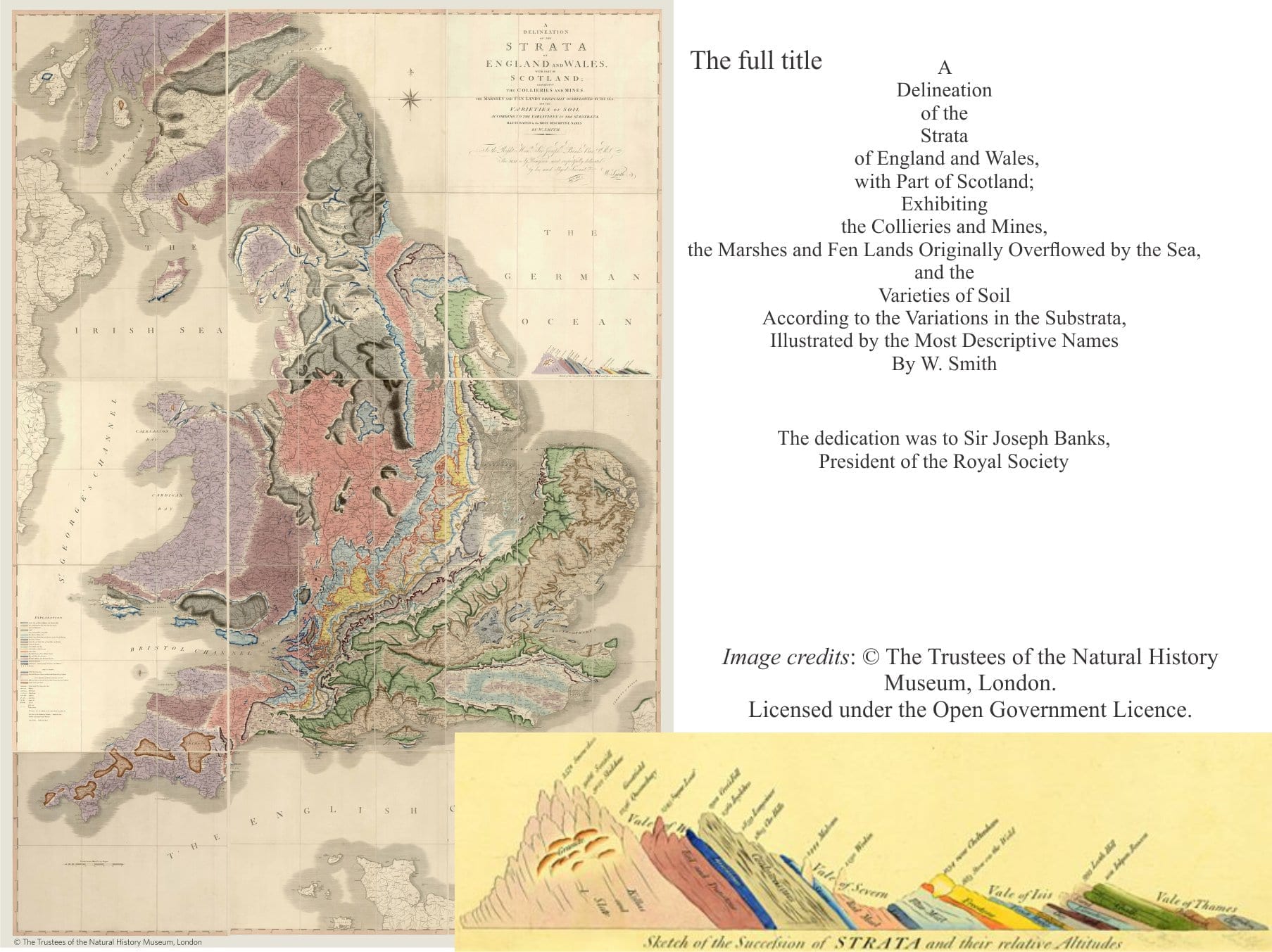
William Smiths map published in 1815 – the one that Changed the World: https://www.nhm.ac.uk/discover/first-geological-map-of-britain.html
“It was the work of genius, and at the same time a lonely and potentially soul-destroying project. It was the work of one man, with one idea, bent upon the all-encompassing mission of making a geological map of England and Wales” (quoted from Simon Winchester’s excellent account, 2001, p.195). The Map, the one that changed the world, was published on August 1, 1815. Four hundred coloured copies were printed, of which only a few remain. It almost covers an entire wall at about 2.6m high, and 1.9m wide. Its compilation required years of exhausting and costly field work – Smith was not a wealthy man, nor of gentlemanly status. He covered more than 130,000 square kilometres mapping and measuring, collecting thousands of fossils. His rock units, many of which were well known, were defined by lithology and fossil content – fossils were particularly important for correlation. Much of the original work was undertaken while surveying new canals.
The beauty of the Map lies in its artistry, the intellect behind its construction, and the important scientific and technological advantages of being able to see, at a glance, the geology of an entire county or country. I have seen one of the surviving copies in the Geological Society (London) foyer. It is stunning.
Upon publication, William Smith was celebrated, at least for a brief period. But the undercurrent of insults and condescension, and an even worse indignity, plagiarism, continued. However, a degree of fortune was to return in 1831 when he was celebrated as the first recipient of the Geological Society’s Wollaston Medal. In his delivery speech, Adam Sedgewick (in important personality in 19th century English geology) even referred to him as the Father of English Geology.
Charles Lyell (1797-1875)
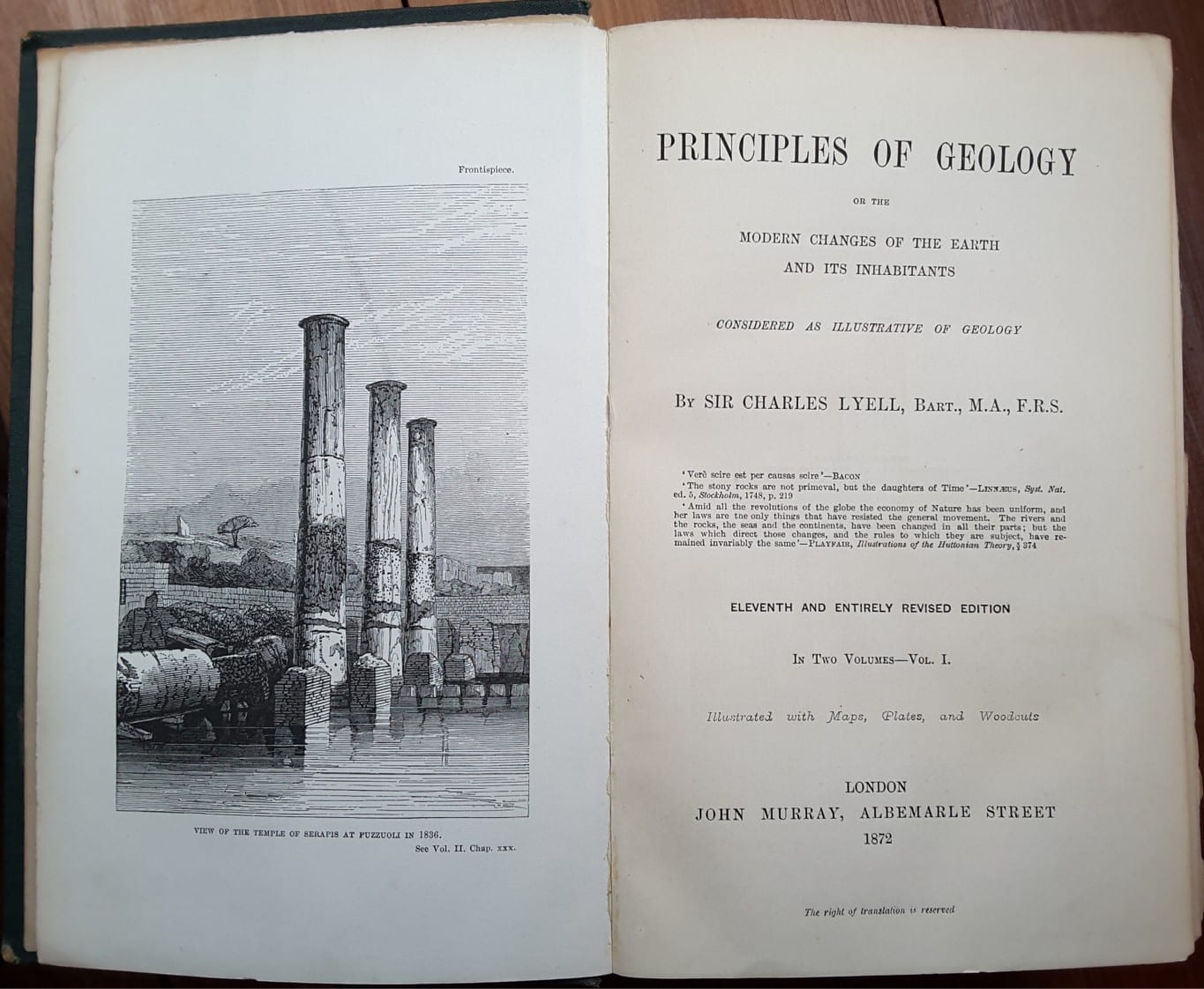
Frontispiece (Roman Temple of Seraphis in Pozzuoli) and title page to Lyell’s Principles of Geology, in the 11th Edition 1872.
Lyell was a quintessential Victorian gentleman (later a Baron), lawyer, and the most influential geologist of the time. He championed Hutton’s uniformitarianism and deep time, providing a Gradualist’s antidote to the prevailing Catastrophism. For Lyell (and Hutton) the upheavals and contortions of the Earth required time beyond reckoning. Although he could remove himself from these Catastrophist reckons, he was acutely aware that some Earth processes can occur rapidly in a geological sense. The frontispiece to Volume 1, the Roman Temple of Seraphis in Pozzuoli (near Naples) illustrates his ability to decipher geological events; the temple columns, partially submerged in 1828 when he observed them, contain clusters of bivalves about 2.7m above the water line. He deduced that the columns must have been almost fully submerged, and later uplifted. In fact, today they are more than 3m above the water line.
His first edition of The Principles of Geology was in 3 volumes, the 1st edition published 1830-33. They constitute one of the first set of texts that deals with pretty well everything geological – from sedimentary to igneous and volcanic processes, earthquakes, the uplift of mountains and the erosion that wore them down, fossils, climate, past glaciations. These weighty tomes were hugely influential to young Charles Darwin who obtained copies during his time on the Beagle (December 1831 to October 1836. Lyell was later to become a good friend and arm-twister to Darwin.
Elizabeth Carne (1817-1873)
Carne combined banking and philanthropy with her love of geology, the latter undertaken in Cornwall. She published four papers in the Royal Geological Society of Cornwall Transactions (she was the first female member elected to this society), including one that reveals a description of ancient sea levels; Cliff Boulders and the Former Condition of the Land and Sea in the Land’s End district. She identified features of the boulders that were like modern deposits along the Land’s End shore, but elevated well above the present shoreline. She was well read, but I cannot ascertain whether she was conversant with the Hutton or Lyell texts. Regardless, her interpretation of the boulders as an ancient beach, formed at a different relative sea level, shows interpretive skills that extended beyond the standard diluvian dogma.
Florence Bascom (1862-1945)
Florence Bascom’s contributions to geology and stratigraphy were numerous, but key among them were her pioneering efforts in developing microscopy as a tool for unraveling rock histories (petrology), and a love of teaching that culminated with her founding the geology department at Bryn Mawr College in Pennsylvania. She applied the principles of crystallography and petrography to sedimentary rocks, having learned the skills studying crystalline rocks. An ability to extend these skills enabled her to decipher sediment provenance, and to distinguish between metamorphosed rocks and non-metamorphosed sediments (this was the topic of a dissertation). She became an expert in Appalachian geology. Microscopy in all its forms continues to play a vital role in many facets of geology.
She earned four degrees, the final one a PhD at Johns Hopkins University in 1893 – not only the first geology doctorate, but the first woman to earn a PhD there. Bascom was the first woman to be hired as a geologist by the U.S. Geological Survey, and the first woman to be elected to the Geological Society of America in 1924.
Johannes Walther (1860-1937)
Walther was a German geologist who gave us The Law of Correlation (or Succession) of Facies, published in 1894 (and translated from German by Gerald Middleton 1973). He became a student of science and geology at a young age (12-15), one of his early mentors being Ernst Haeckel, a biologist, a Darwinist, and brilliant illustrator of living and fossil organisms.
His investigations involved marine geology, comparisons of modern and ancient sedimentary processes (uniformitarianism), was one of the earliest to recognize bioerosion as a significant source of carbonate sediment, and established that coral reefs had rigid frameworks plus interstitial sediment. Later in life he became a professor and dean (Gischler, 2011).
We remember Walther primarily for his ‘Law’, that is an essential part of any modern analysis of sedimentary facies and depositional systems (most English-speaking students will only be familiar with Middleton’s translation and commentary.
‘‘. . . only those facies and facies-areas can be superimposed primarily which can be observed beside each other at the present time’’ (Walther 1894). Stated another way Walther’s Law indicates that facies that form coevally in laterally contiguous environments can be superposed vertically. It is possible that Walther was pre-empted by Lavoisier’s analysis, but Walther was the first to formally state the condition for facies disposition.
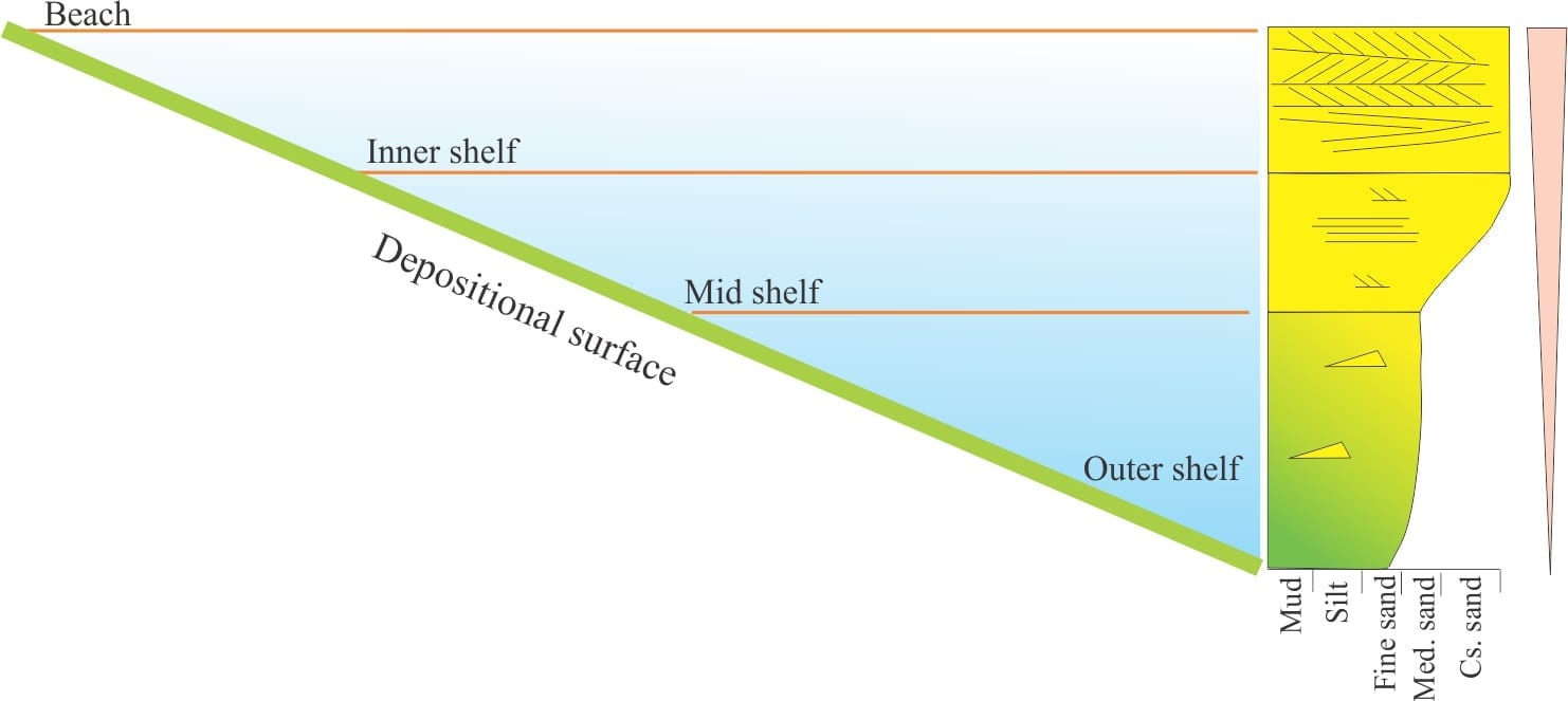
An illustration of Walther’s Law. The deposits encountered on a transect across the shelf are represented stratigraphically in the coarsening upward succession
The example shown depicts a traverse from beach to outer shelf, with concomitant changes in sediment (particularly grain size and sorting), benthic fauna and flora, and sedimentary structures. Assuming no significant interruption, the facies progression will be translated to a hypothetical stratigraphy, in this case under conditions of regression and seaward migration of the shoreline.
Eliot Blackwelder (1880—1969)
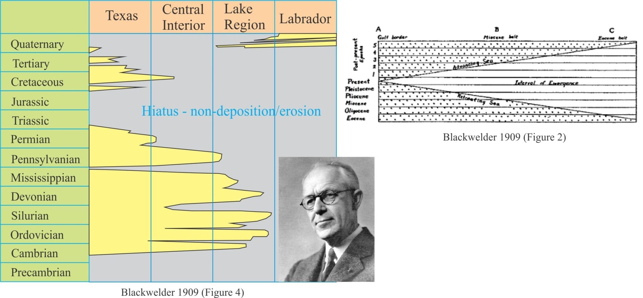
Blackwelder was essentially a field geologist, known for his scrupulous attention to detail and observation, as broad-based in his interests as any Victorian gentleman naturalist. There are several reasons why his inclusion in the timeline is warranted, but key among them is a paper on unconformities published in 1909. He was the first to identify continent-wide successions of Phanerozoic strata, each separated by profound unconformities. We now refer to these successions as sequences.
Blackwelder’s continent-wide unconformity bound successions and illustration of regression and transgression provided the conceptual impetus for later geologists like Larry Sloss, David Frazier, and Peter Vail
His Figure 2 is one of the earliest graphical portrayals of the chronostratigraphic significance of unconformities. The stratigraphic succession at A is continuous, but from B through C the duration of missing time increases, that he attributes to erosion of the rock record. The rise and fall of sea level (transgression and regression), and concomitant landward or seaward migration of the shoreline, produces a mappable contact that is diachronous. The diagram on the right is remarkably similar to Grabau’s 1906 Figure 7.
His scheme of unconformity-bound successions was expanded by Larry Sloss in 1949.
An excellent publication by Andrew Miall (2016) revisits Blackwelder’s unconformities, evaluating them in a more recent context.
Joseph Barrell (1869-1919)
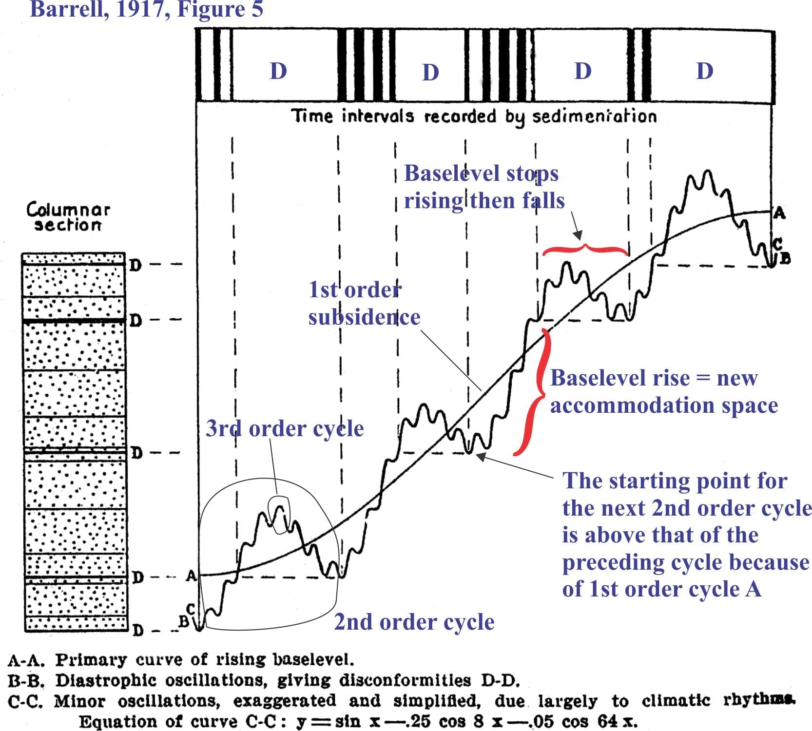
Barrell’s interests extended from the global (heat production, isostasy) to the origin of sedimentary facies and depositional rhythms, or cycles. His classic paper on cyclicity (1917; a 159 page tome) considered stratigraphic rhythms and rates of denudation and sedimentation. He portrays these cycles in the context of changing baselevels, one of the first explicit explanations of the value of a datum in stratigraphy. His Figure 5, that could be transposed to any modern publication on changing sea levels, shows the effects on sedimentation from harmonic oscillations in baselevel.
Barrell’s 1917 diagram is a remarkably modern take on the relationship among base level cycles, deposition and non-deposition (diastems). Annotations in blue are mine. Modified from Geological Society of America Bulletin v.28
The diagram models:
The long-term change in baselevel caused by subsidence (curve A),
Long-period oscillations, or 2nd order cycles caused by tectonism, and
Short period (higher order) cycles caused by fluctuating climate.
Higher order cycles are superimposed on long period cycles; we certainly know this to be true, for example Milankovitch astronomical cycles that drive oscillations in climate. Barrell then correlates changing baselevels with the deposition of sediment, and periods of little or no sedimentation that he calls diastems (D on the stratigraphic column) caused by a reduction in sediment supply and/or erosion. The corresponding time intervals are shown in the top bar – solid black lines represent sedimentation, blank spaces represent diastems.
Barrell’s diagram further illustrates:
Stratigraphic columns may appear to represent continuous sedimentation, but in fact they contain long periods with no sedimentation.
Whether sedimentation or diastemic breaks occur depends on the overall effect on baselevel of all three cycles, and
Sedimentation only occurs when the overall baselevel is rising. In other words, when there is space to put sediment. We now refer to this as accommodation space. In his own words “…the deposition of nearly all sediments occurs just below the local baselevel represented by wave base or river flood level, and is dependent on upward oscillations of baselevel or downward oscillations of the bottom, either of which makes room for sediments below baselevel.” (p. 747). Some of the jargon has changed, but this is essentially a modern statement about baselevel controls on sedimentation.
Amadeus William Grabau (1870-1946)
Grabau was an American paleontologist who, in addition to important work in continental USA, also spent a significant part of his life in China. Of his many books, three that deserve mention here are On theClassification of Sedimentary Rocks (1904), Principles of Stratigraphy (1913), and importantly Rhythm of the Ages (1940) where he elaborates on his pulsation theory (a theory introduced in 1933 at the International Geological Congress, Washington).
The Pulsation Theory attempts to explain the repetition through time of strata having similar sedimentary and paleontological attributes. Repetition of these successions of strata, more commonly known as cycles and cyclicity, resulted from successive marine transgressions and regressions (about 20 years after Barrell’s model if cyclicity). Grabau was one of the first exponents of Global Eustasy, where advancing seas were caused by expansion of the oceans, and vice versa retreating seas. From his correlations of Phanerozoic stratigraphy, he reconstructed continental paleogeographies that were also consistent with Alfred Wegener’s ideas on continental drift.
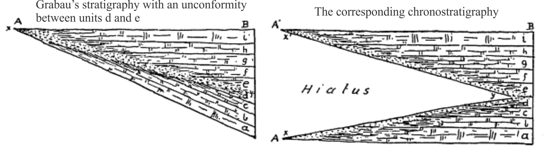
Grabau extended Walther’s Law, recognizing that there are gaps in time caused by sedimentary processes, particularly erosion during shoreline seaward retreat. He coined the term hiatus to describe the absence of a rock record between pulsations, or cycles. The diagram below from Figure 7 of a 1906 publication shows a stratigraphic (left) and corresponding chronostratigraphic representation; the similarity to more recent diagrammatic expressions of onlap and offlap is striking. Note that this also approximates a sea-level curve.
Grabau’s 1906 chronostratigraphic illustration of transgression and regression, separated by an hiatus. From Geological Society of America Bulletin, v.17.
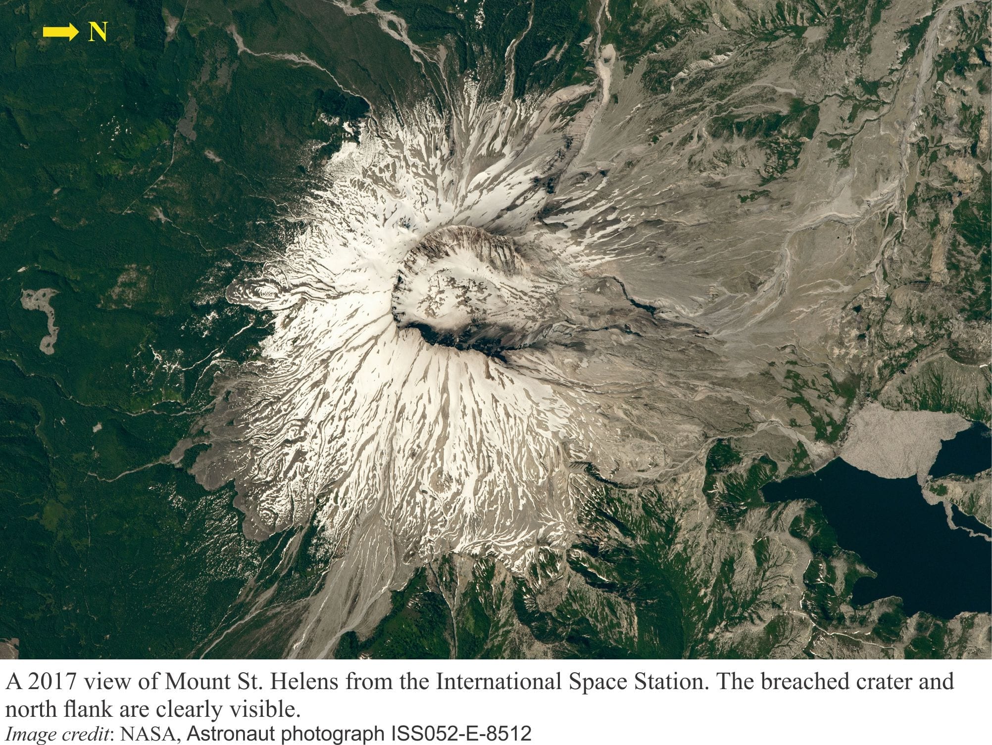
May 18, 1980, a crisp, clear Cascade mountains morning was rent by the catastrophic eruption of Mount St. Helens. Fifty seven people were killed by the initial eruption blast. Lives and landscapes were changed irrevocably.
Mount St. Helens is one of several historically and prehistorically active volcanoes in an arc stretching from northern California to southern British Columbia – about 1100 Km. The first signs of awakening began March 16, 1980 with a burst of seismic activity, followed on March 26 by a small eruption that produced some ash and steam – the first such eruption in 100 years. Small eruptions (small by comparison with what was to follow) continued off and on into May. For the two months prior to May 18, geologists and seismologists monitored the volcano; measuring its earthquakes (1000s of them), the changing shape of its summit, and changes in heat beneath the ground.
Over this period, rising magma caused the north flank of the edifice to bulge – photos taken just prior to the main eruption show dramatic changes in the land surface along this flank. As it turned out, the accumulating magma was acting as a kind of pressure-relief valve. At 8.32 am a magnitude 5.1 earthquake dislodged the intruded magma, causing the northern flank to collapse in a massive landslide. The main body of the landslide was mobile enough to travel 22 km down the adjacent valley.
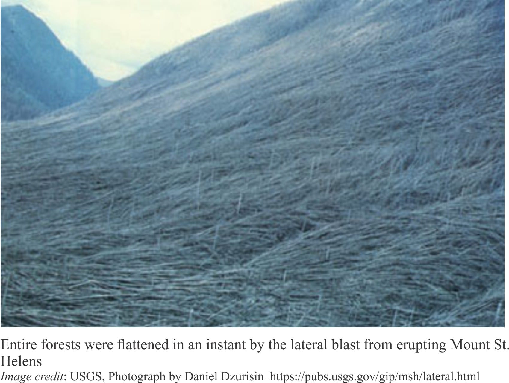
Failure of the north flank effectively opened the vent pressure valve – commentators frequently liken this process to the popping of a champagne cork. Two things happened:
Pressure release across the volcano flank produce a catastrophic blast of hot gas, ash, and large rocky ballistics that moved laterally (this phenomenon is called a lateral blast), flattening everything in its path. The ground-hugging ash flow swept up ridges and through valleys, at speeds up to 480 km/hour.
Within a few minutes the main eruption column had risen 24 km above the Earth’s surface. Some of this ash fell back onto the volcano’s flanks producing pyroclastic flows – albeit smaller flows than the initial lateral blast. Over the next 15 days, ash and aerosols that entered the upper atmosphere had circled the Northern Hemisphere.
Millions of tonnes of ash covered western US states and southern Canada. Debris from the landslide and lateral blast blocked rivers and created new lakes. Subsequent snow melt and rain moved much of the loose ash into rivers, creating new hazards in the form of highly mobile mud flows, or lahars. These kinds of problems continued for years following the main eruption.
The 40th Anniversary of the eruption, the lives lost, and lives changed, are remembered in webinars, documentaries, old footage and images, by scientific organizations and the media (mainstream and social). I have listed a few below.
Some links to really good MSH resources:
TheUnited States Geological Survey was and remains a key player in volcano monitoring. 40 Years Later: The Eruption of Mt. St. Helens and the USGS Response: Overview
The Smithsonian Institute has an excellent list of webinars and activities that will appeal to all ages and interests
NASA Earth Observatory has some great images of Mt. St Helens from various satellites and the International Space Station
Voices of Volcanology is a Facebook group dedicated to keeping everyone updated on volcanoes, volcanic activity, and myth-busting (like all those stories on the Yellowstone supervolcano). Here is a great example where Janine Krippner interviews Dr. Seth Moran, the scientist-in-charge of the Cascades Volcano Observatory.
The history of science is littered with the misplaced contributions by women, contributions that at best were pushed aside or ignored, and at worst thought of as shrill outbursts. Witness:
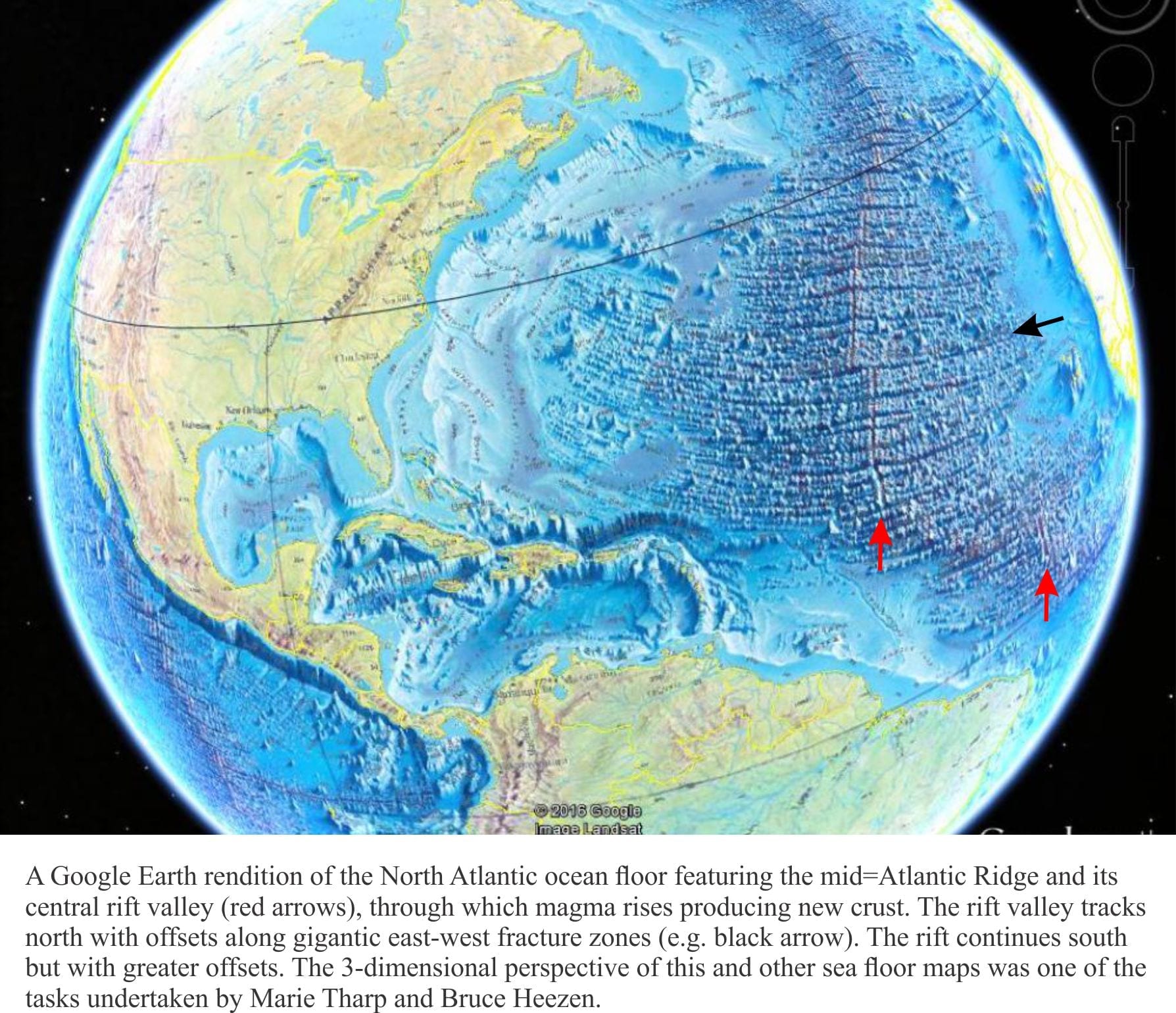
as corrections to a history where women found it difficult to escape the status of ‘footnote’. We can add Marie Tharp (1920-2006) to the growing list of corrections. In 1952 Tharp discovered the central rift system in the mid-Atlantic Ocean ridge (that later would become a critical component of sea floor spreading and plate tectonics) but for many years was regarded as a minor player in the burgeoning, post-war field of oceanography.
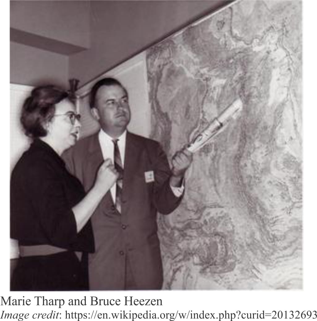
During the War, Tharp in her early twenties took advantage of opportunities to engage in university study, openings in science and engineering left by men who had gone to battle. She completed a Master’s degree in geology, but given that geology is a field-based discipline, and that women weren’t supposed to go into the field, she extended her studies to a Master’s in mathematics. In 1948 Lamont Geological Laboratory (now Lamont Doherty Earth Observatory) hired 28 year-old Tharp to draft maps of the Atlantic ocean floor, based on the growing database from SONAR and historical soundings. She worked with well-known geologist-oceanographer Bruce Heezen, who spent much of his time at sea. It must have been tedious work, but she counted herself lucky to have a position at all. This was a time when very few American universities (or anywhere else for that matter) offered science and engineering positions to women; a time of patriarchal condescension – “Mad Men” versus “Hidden Figures”.
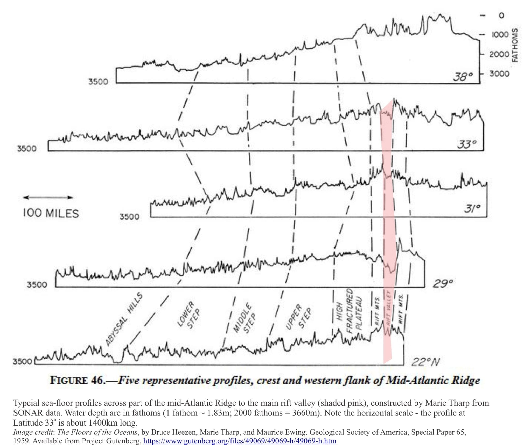
Tharp poured over depth and positional data for years, constructing 2-dimensional profiles of the Atlantic Ocean floor. She was aware, as other oceanographers were that an elevated region of sea floor apparently separated east and west Atlantic. This was initially mapped in 1854 by US Navy oceanographer, geologist and cartographer Matthew Maury, and later confirmed with depth soundings taken during the HMS Challenger expeditions (1873-1876 – Challenger had 291 km of hemp onboard to do this kind of thing; the ridge is generally deeper than 2000m). Tharp wasn’t surprised to find the Atlantic ridge on her profiles. What did catch her attention was the rift-like valley in the central part of the ridge; a geomorphic structure that was consistent through all her profiles. She immediately recognized the importance of this, because it implied significant extension, a pulling apart of Earth’s crust in the middle of the ocean. At the time, the general consensus was that ocean floors were relatively benign, featureless expanses. Her discovery indicated otherwise.
According to Tharp’s bio the response by Heezen and his colleagues was that she was being a typical woman – you know, “girl talk”. One can imagine the coffee room banter; ‘she’s great at drafting cross-sections but should leave the interpretation to the more learned’.
However, after some months and more profiles all showing the same rift- like structure, Heezen gradually accepted that this was real. A turning point for Heezen was the coincidence of several mid-ocean earthquake epicenters along the ridge. This was mid 1953. He understood its potential significance, particularly for those who thought that the hypothesis of continental drift had some credence (Heezen was not initially one of those people).
Ocean bathymetry studies in other basins in the early 1950s (Indian Ocean, Red Sea) revealed similar mid-ocean rifts. Tharp had by this time surmised that a rift valley coursed its way almost continuously the entire length of North and South Atlantic, a distance of 16,000 km; it was the largest continuous structure on Earth. The Lamont Doherty group gradually realized that the Atlantic structure, together with those discovered in other ocean basins, represented a gigantic Earth-encircling system of mid-ocean rifts, more than 64,000 km long.
Heezen presented their research to a 1956 American Geophysical Union conference in Toronto. Marie Tharp barely received a mention. She did co-author a few subsequent publications as an ‘et al.’, but it was a kind of ‘also ran’; the accolades and approbation went Heezen’s way.
Tharp was fired by the Laboratory, the victim of a spat between Heezen and Lamont boss Maurice Ewing, but she continued to develop the maps at home. Marie continued to work in the background, as the humble and grateful recipient of a job she considered to be fascinating; “I worked in the background for most of my career as a scientist, but I have absolutely no resentments. I thought I was lucky to have a job that was so interesting”.
Marie Tharp was named one of the four great 20th century cartographers by the Library of Congress in 1997, was presented with the Woods Hole Oceanographic Institution Women Pioneer in oceanography Award in 1999, and the Lamont-Doherty Heritage Award in 2001.
There is no question that Tharp’s discovery influenced the promotion of Continental Drift in the geoscience community. Alfred Wegener’s bold hypothesis (1915) had one major problem – there was no known mechanism that could move oceanic crust and continents around, like some precursor shuffle to a jigsaw puzzle. In 1929 Arthur Holmes posited a mechanism that involved large convection cells in the mantle, but this too lacked an important degree of empirical verification. Discovery of the mid-Atlantic rift provided a solution to this vexing problem, and in 1962 Harry Hess proposed that new magma, via mantle convection cells, was erupted from mid-ocean rifts allowing oceanic crust to spread outwards. This was Sea Floor Spreading, a precursor to the grand theory of Plate Tectonics – the tectonic shift in geological thinking wherein oceanic crust is created at mid-ocean rifts and consumed down subduction zones, with the continents playing tag.
Marie Tharp’s doggedness in her belief and understanding of mid-ocean rifting is now celebrated. It’s taken a few decades, but she is no longer a footnote.
We are regular visitors to the beach; walks with the kids-grandkids, the dog, swimming, fishing, or just sitting and cogitating. It’s easy to get lost in the timeless rush of waves, their impatient foam. My mind reels at the thought that the sea has been doing this for more than 4 billion years. It’s a bit like getting lost in the night sky. There’s so much to discover.
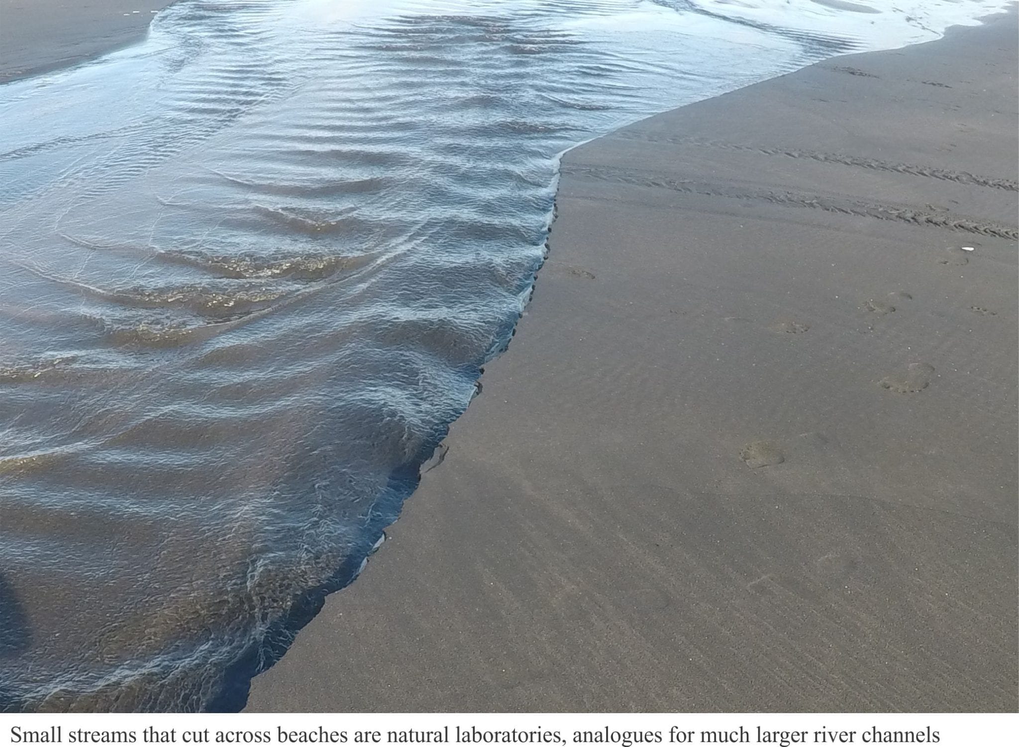
Beaches are geological domains – part of a continuum that extends to the deep ocean, but a part that is easily accessed. Geological stuff happens there. My attention is always grabbed by the small streams that drain across beaches at low tide. Whenever we came across one of these my kids would scatter, lest they be regaled yet again about the fascination of miniature worlds. I admit it was a bit over the top, so it goes…
Some beach outflows come and go with the tides, others are more permanent leakage from inland drainage. Some trickle, others rush. They are all fascinating, as microcosms of grander floodplain or massive deltas. Project this microcosm to the real world of geological process, of cause and effect. In doing this, you are engaging in the scientific process of creating your own analogy, an insight into a larger universe.
The streams usually start afresh with each tidal cycle. As tides recede, stream flow begins to erode its channel, deepest at the top of the beach. The channels may be straight and narrow, or broad networks of braided sand. Continue reading →
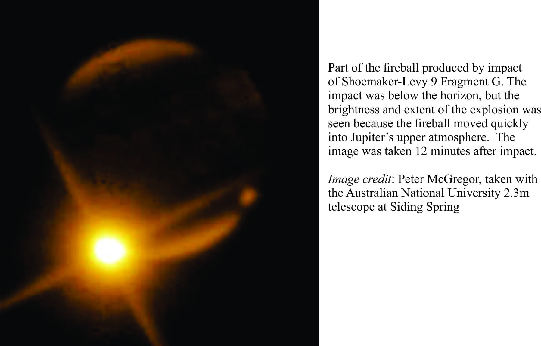
The dinosaurs were snuffed out in a geological instant (well not exactly, but that is a popular image). The Chicxulub bolide, its girth 10-15 kilometres, collided with Earth 65 million years ago, leaving a 150 kilometre-wide crater and enough dust and aerosols in the upper atmosphere to darken latest Cretaceous skies for decades.
Like all planetary bodies in our Solar System, Earth has received its share of meteorite and comet impacts. We still bear the scars of some. Every day, bits of space dust and rock plummet towards us – most burn up on entering the atmosphere, but a few make it to the surface. Occasionally they even startle us with air-bursts – Tunguska in 1908, Chelyabinsk (2013), both in Russia. But humanity has never witnessed a decent sized impact, at least in recorded history. It’s all theoretical. Continue reading →
A safe harbour offers a place of refuge. Those in peril (or evading taxes), running before a storm, crossing a figurative bar to welcome respite. Non-figurative harbours, the coastal kind, have traditionally provided safe haven for mariners escaping inclement weather or foes.
Harbours fill and are emptied of seawater on the tide. Sea water that enters or exits is commonly focussed through narrow inlets. Here, powerful currents are generated that carry fish, sediment, flotsam, and unwary boats. Filling on an incoming tide is like a cleansing, a renewal; outgoing tides reveal channel arteries that keep alive the bars and broad flats of mud and sand, textured Kandinsky-like.
Northern New Zealand’s west coast has 6 harbours distributed along a 300 km stretch of coast. Each is protected by large sand barriers that have built over the last 2-3 million years with sand moved inshore by successive rises and falls of sea level.
Many of New Zealand’s harbours are drowned valleys, where rising sea level (following the last glaciation) has inundated dissected landscapes. Rising seas have crept up valleys, leaving the exposed high ground to front an intricately embayed coastline, islands, and estuaries that extend their marine fingers far inland.
New Zealand’s west coast is open to large swells, generated by westerly winds across a 2000 km expanse of Tasman Sea. Sea conditions along this coast are often rough. Access to the open sea via harbour inlets, requires sailors to ‘cross the bar’ – the zone of shallow, constantly moving sand. Strong tidal currents, particularly out-going tides can increase wave heights even further, as well as making wave conditions in general very choppy. The sea condition can change rapidly. Many a boat has come to grief across these west coast bars, a mix of bad luck and poor judgement (NIWA has real-time images of current bar conditions at several locations).
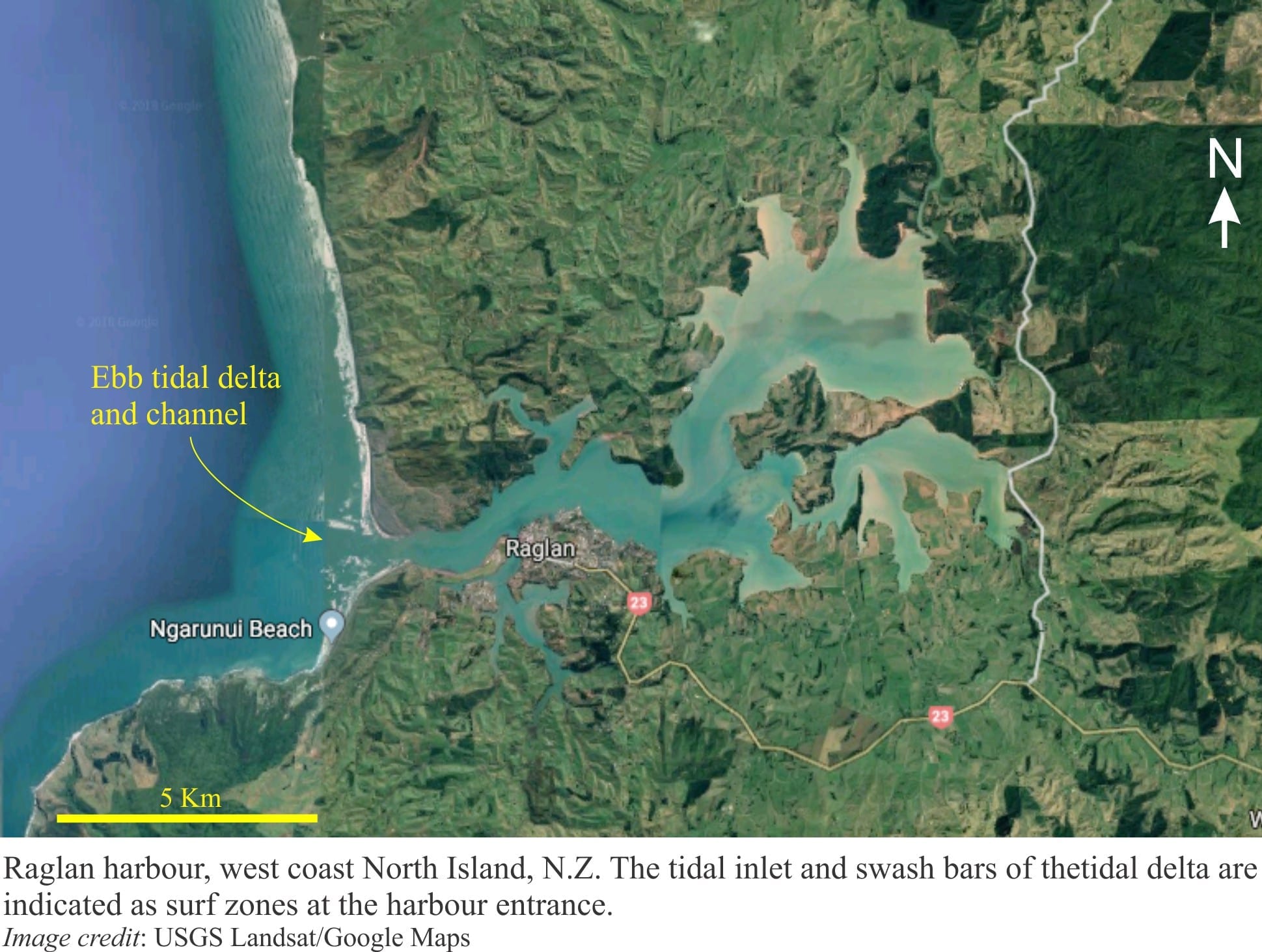
The oceanographic and geological term for sand bars at the entrance to harbours and lagoons is tidal delta. Tidal deltas can form on the seaward margin, in which case they are called ebb tidal deltas (because they are downstream of the outgoing tide). Those that form inside harbours and lagoons are flood tidal deltas where sand is deposited by incoming tides.
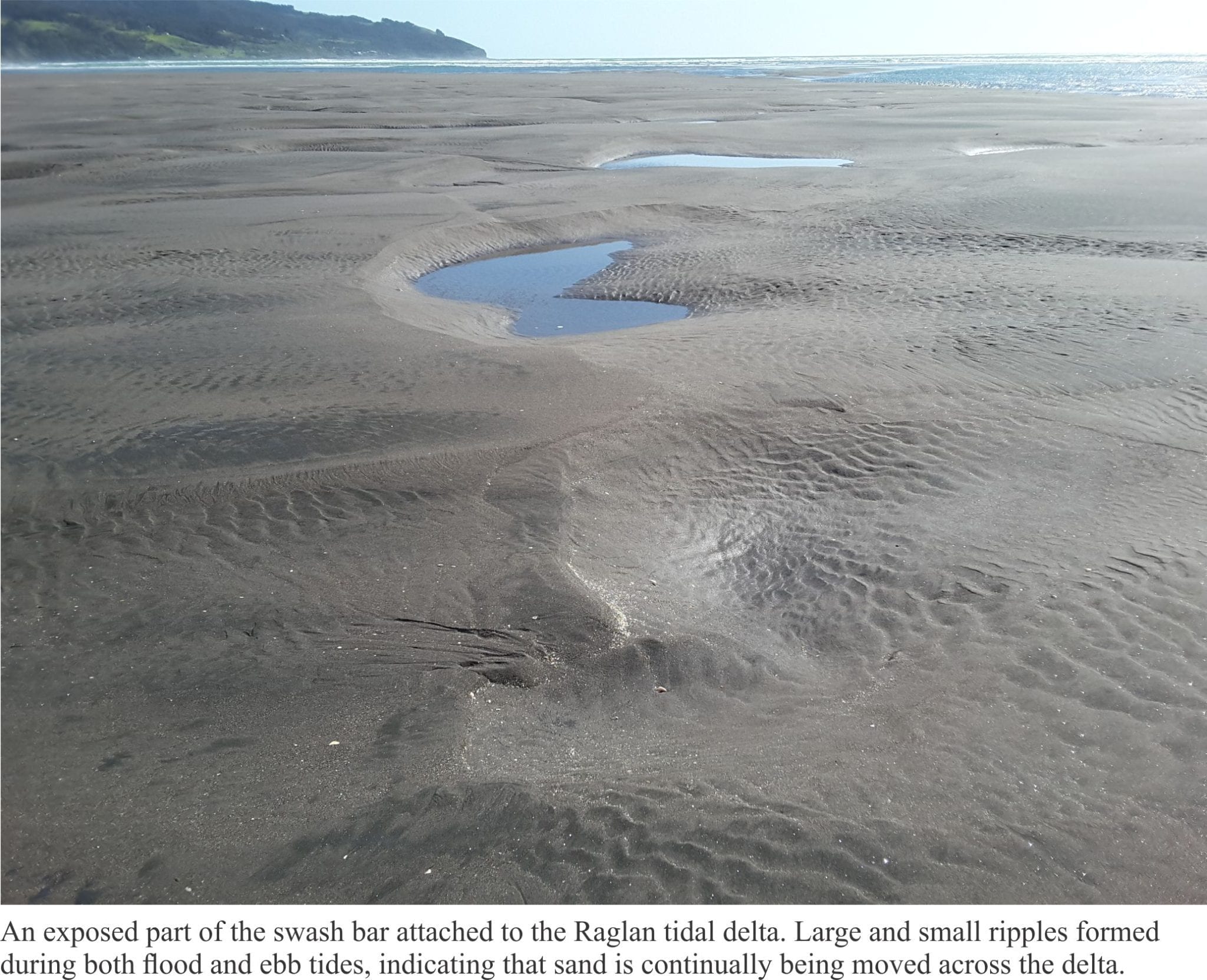
Raglan Harbour is small but it sports a very nice example of a symmetrical ebb tidal delta. The delta extends 1.5 – 2 km from the harbour mouth. Darker hues (image below) that mark the main channel contrast nicely the shallower sand bars on either side over which waves tend to break. These marginal sand deposits are called swash bars.
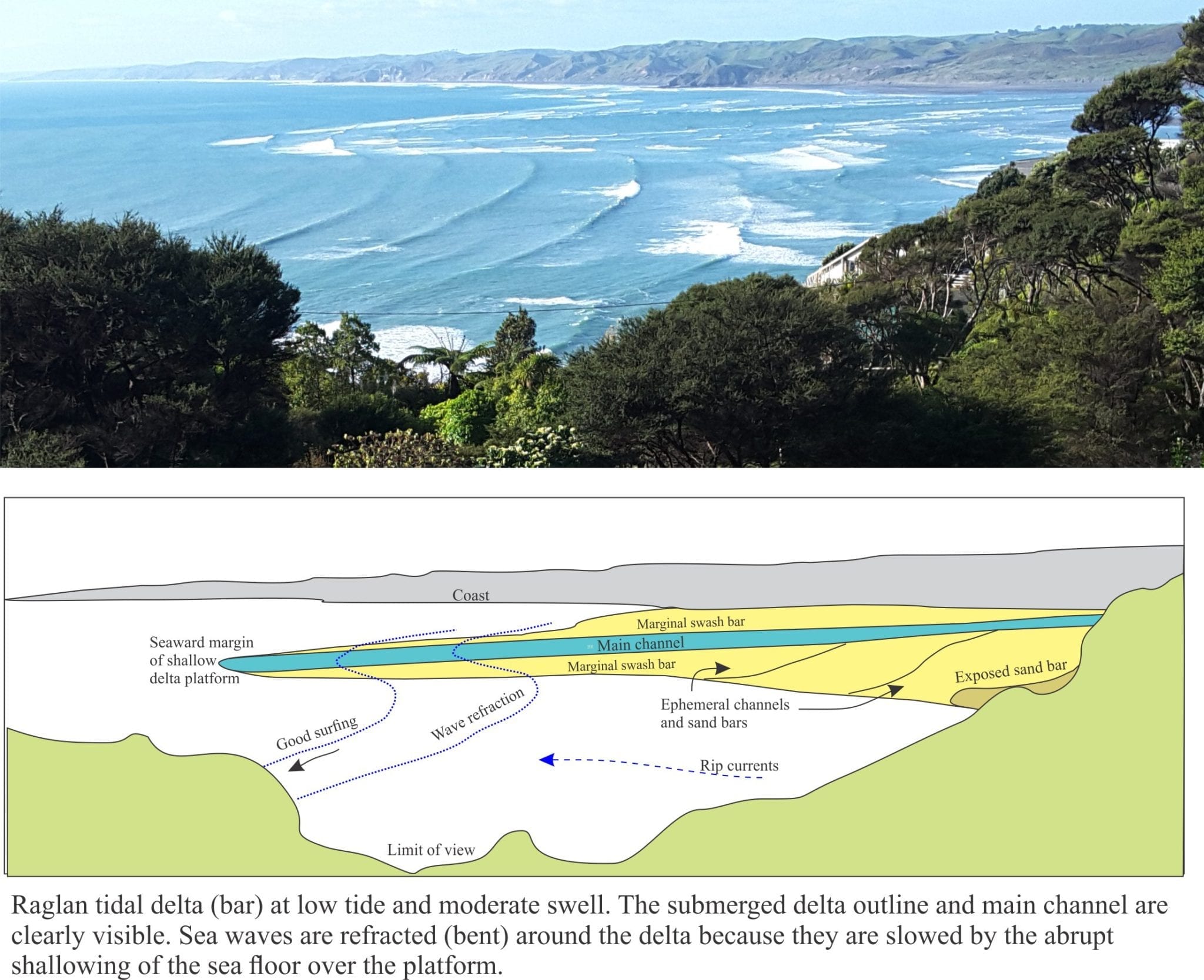
Westerly swells approach the coast with relatively straight crests. As they pass over the shallow delta platform, they move at a slower speed because they interact (friction) with the sea floor. Some of the wave energy is transferred to the sea floor such that sediment is moved as ripples and dunes. Slowing waves also build in amplitude (height); this is the region where waves break. However, the same waves in the adjacent, deeper water are moving at a faster pace – trace the crests of each wave and you will see it ‘bending’ around the delta.
Most of the tidal delta remains submerged even at low tide. Parts of the swash bar that are exposed during low tide show evidence for sand movement, mostly as ripples, large and small. Sand is moved during flood and ebb tides. The shape of these sand bars changes from one tide to the next, demonstrating that this is a dynamic environment.
The Raglan tidal delta consists almost entirely of sand. In contrast, Raglan Harbour and its estuaries contain a high proportion of mud. So where does all that sand come from?
The tidal delta is part of a much larger system of sand transfer – supply and demand from the adjacent continental shelf to the adjacent beaches, shallow sand bars (commonly formed by rip currents) and sand dunes. Sand in the inshore region is also moved along the coast by long-shore currents and it is this sand that continually feeds the delta. The delta in turn, via its main channel, moves sand back onto the shelf, completing the cycle.
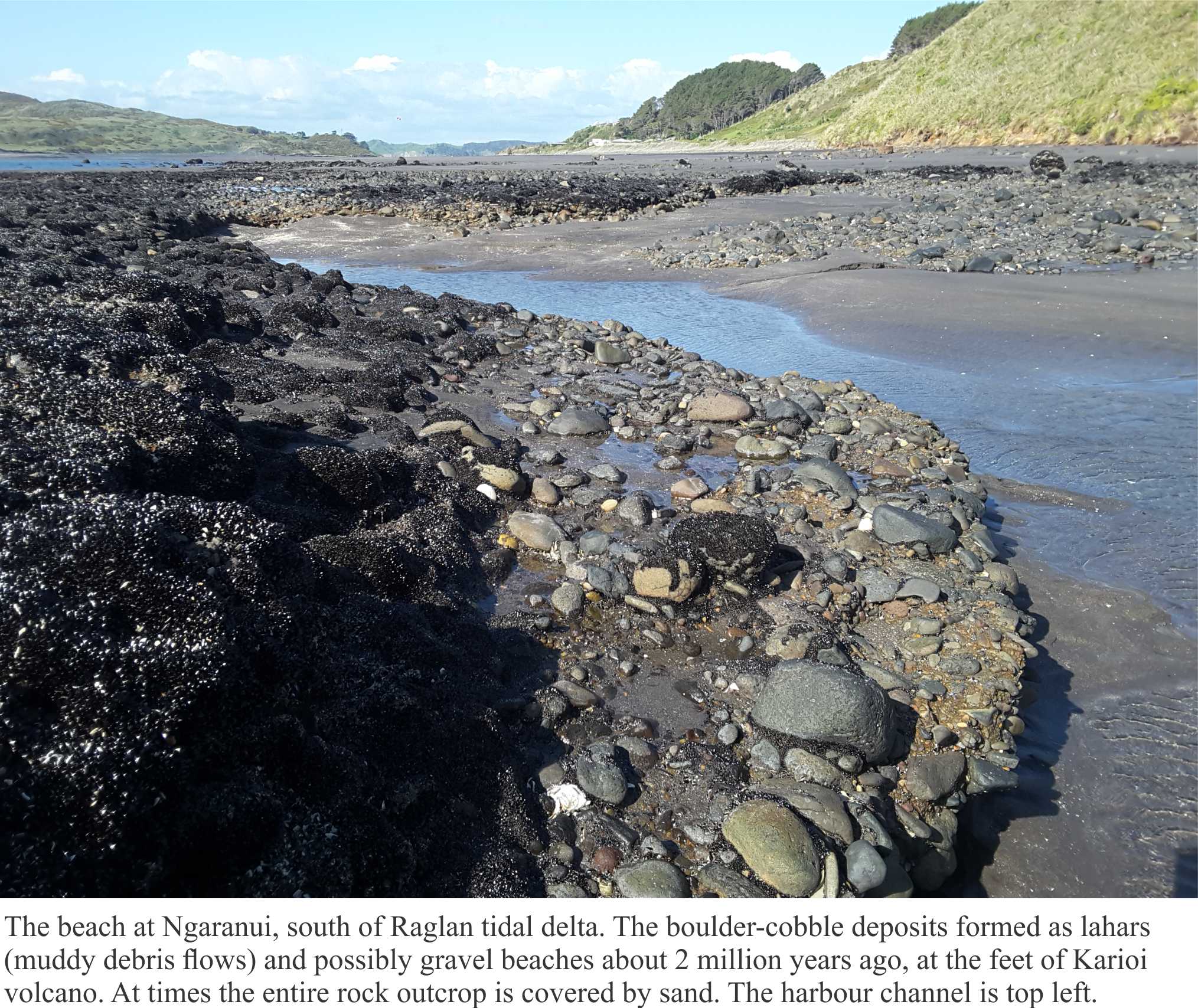
The beach south of the tidal delta continually changes its profile. At times the profile is an uninterrupted swath of black sand along most of its length (about 3 km). At other times a significant volume of sand has been removed exposing ancient boulder deposits from nearby Karioi volcano; sand removal frequently occurs during stormy weather. The sand dunes also participate in this budgeting exercise. Sand transfer from the beach (and dunes) is probably a combination of movement directly offshore by rip currents and wave undertow, and long-shore movement towards the delta. Sand replenishment and removal from the beach, and addition to the tidal delta, is part of a much larger system of sand supply and demand – nature’s sand budget.
Sand moved onto the swash bars helps to replace sand that is removed by the deep, fast-moving channel. Channel flows in narrow inlets like the one at Raglan are commonly 4-6 km/hr (1-2 m/second), which may not sound fast (try swimming against it) but is sufficient to move large volumes of sediment during each tidal cycle. There are some small sand bars in the harbour itself, but the channel is an effective flushing mechanism that prevents the estuaries and tidal flats from clogging up.
Changes in sea level have a profound impact on coastal sand systems. If sea level falls, the beach and dunes would follow the retreating shoreline, the harbour would eventually become the domain of non-tidal rivers and swamps, and the main channel would be free to meander over a broad expanse of exposed continental shelf. Tidal deltas might be more ephemeral structures, constantly on the move. This was probably the scenario during the last glaciation, when sea level was more than 100m below its present position.
Perhaps of more immediate concern is a rise in sea level (the present situation) which would erode older foreshore beach and dune deposits, and destabilise some cliff areas south of the Harbour. The Surf Club at the south end of Ngarunui Beach would need to move – yet again. The Harbour area flooded at high tide would increase, resulting in a greater volume of seawater entering and exiting the narrow inlet. To accommodate this, the inlet would need to expand, or the speed of current flow would need to increase. Changes such as these would have an immediate effect on the size and shape of the tidal delta.