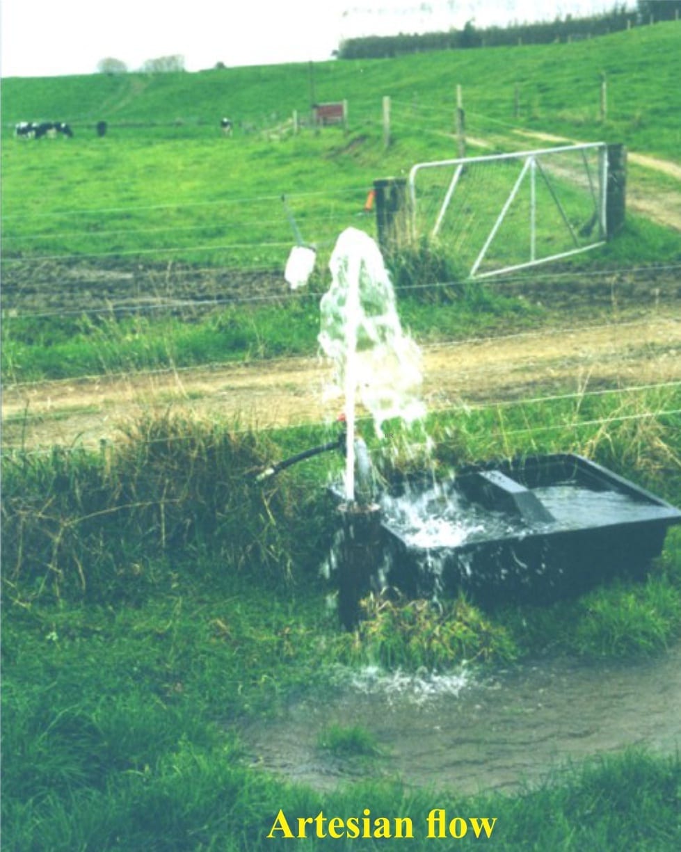
Artesian flow
Henry Darcy’s pivotal experiments with sand-filled tubes (in 1856) established an empirical relationship between hydraulic gradient (that is basically an expression of the hydraulic potential energy available for flow) and discharge. A modern rewrite of the basic equation that he deduced from experiments, the eponymous Darcy’s Law, is:
Q = -KA(Δh/D) where (1)
- Q is discharge (that has dimensions L3/T),
- K is a proportionality constant, subsequently called the hydraulic conductivity (L/T)
- A the cross-section area of a flow tube (L2) (Q is also proportional to A), and
- Δh/D the head difference between two locations along a flow path, at distance D. Note that hydraulic head h is the sum of the pressure head and elevation head.
The hydraulic conductivity (a term borrowed from electrical theory), has dimensional units of distance and time (commonly expressed as cm/s, feet/s). Thus, in mathematical terms, K is expressed as a velocity, also known as the Darcy velocity.
Darcy’s empirically derived law is pivotal to modern, quantitative hydrogeological modelling. The description of his experiments and derivation of the law were published in Note D, an appendix to a lengthy report on the Dijon Fountains (680 pages!): Les Fontaines Purlieus’ de la Ville de Dijon (The Public Fountains of the City of Dijon). While the appendix might seem like an afterthought, it was in fact the culmination of two decades of observation, testing, experimentation, and the creative ability to extend his ideas below the surface, literally and figuratively.
How did Darcy arrive at this point of discovery?
Henry Darcy (1803-1858) was a French engineer who rose to prominence in the 1830s, at least in the public’s eyes, as the designer and executor of a modern water supply system for the city of Dijon, completed about 1840. Several other European cities modelled their own water supply networks on his design. The primary water supply for the Dijon network was a well dug into a groundwater (artesian) spring; the pipe supply network extended 28km – all gravity fed.
Darcy was familiar with the hydraulic theory and practice of the time; the theory of hydraulics was well established but the general understanding of aquifer dynamics was limited. Some of the important ingredients that contributed to his thinking and intuition were:
- Bernoulli’s (1738) mathematical expression for energy conservation during fluid flow; in other words, flow requires an energy gradient. Bernoulli’s equation can be written as:
V2/g + z + P/ρ.g = a constant known as hydraulic potential (2)
where V2/g is kinetic energy, z the elevation head, and P/ρ.g the pressure head. By ignoring the kinetic energy component, that is insignificant for most groundwater problems, the equation reduces to a statement where hydraulic potential is the sum of z + P/ρ.g. The value of this statement is that it allowed Darcy (and us) to tease apart the components of hydraulic head in real wells and experiments.
- He had developed an expertise with the practical problem of pressure losses between the entry and exit points of pipes used to transport water; he surmised and calculated the effects of surface roughness on energy, and therefore pressure losses.
- Another crucial discovery, based on his work with pipes, was that at very low flow rates in small-diameter pipes, the head loss (or head gradient) was proportional to flow rate, that he would later discover could be applied to aquifer flow.
- He was familiar with the flow of water through natural and constructed sand filters that were used to clean river water and was aware that frictional energy losses also applied to this kind of flow.
- He had measured well drawdown for various pumping rates and observed well recovery.
- He had general knowledge of aquifer geology and aquifer recharge by precipitation.
Darcy’s conceptual leap was to equate the physical nature of these observations (in pipes, filters, and the behaviour of boreholes) with flow through porous aquifer media. The experiments he designed and performed bridged the gap between concept and empirical evidence.
Darcy’s experiments
Darcy began his experiments in 1855. They were based in part on his observations of flow through sand filters, but what he needed was a way to quantify head loss (hydraulic gradient).
A diagram showing the original experimental apparatus is reproduced here. Modern groundwater texts commonly redraw the apparatus configuration to be more reflective of aquifer flow – I have added a duplicate diagram.
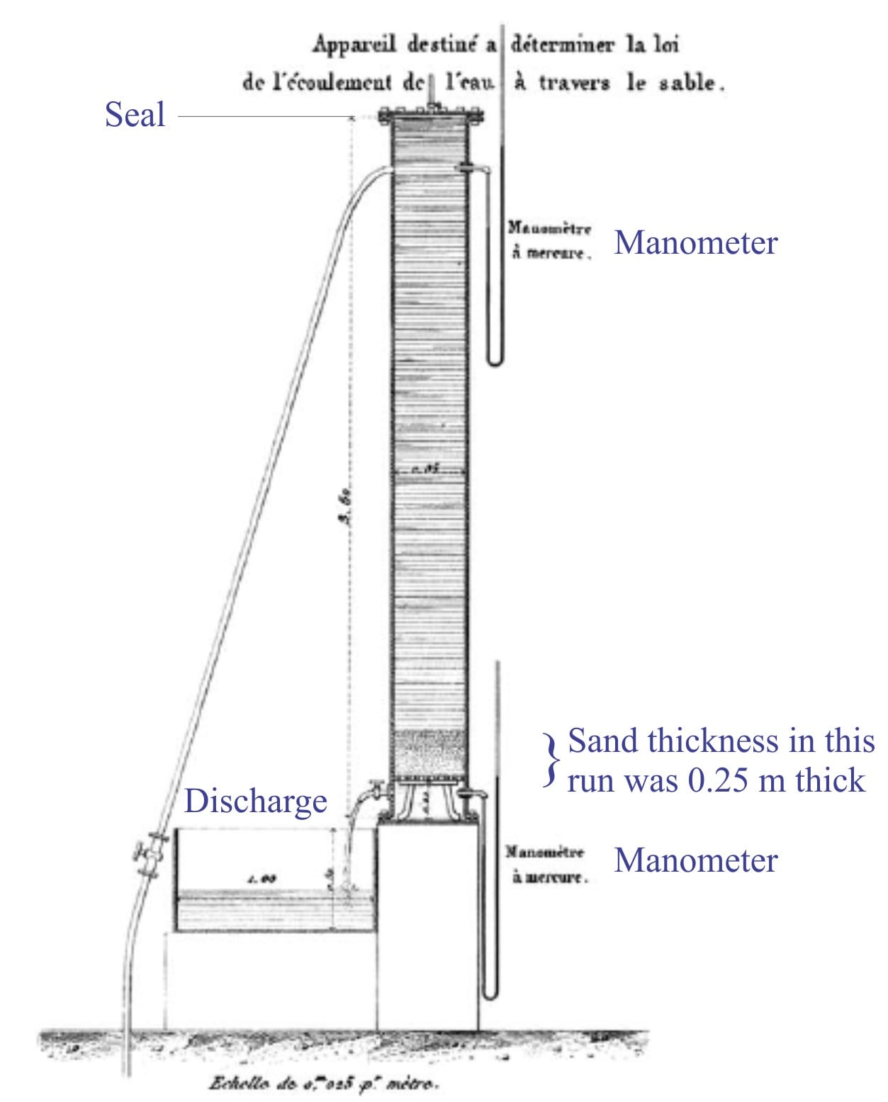
Darcy’s apparatus for determining the relationship between aquifer discharge and head loss, 1856. Figure 3 Plate 24, with some additional annotation
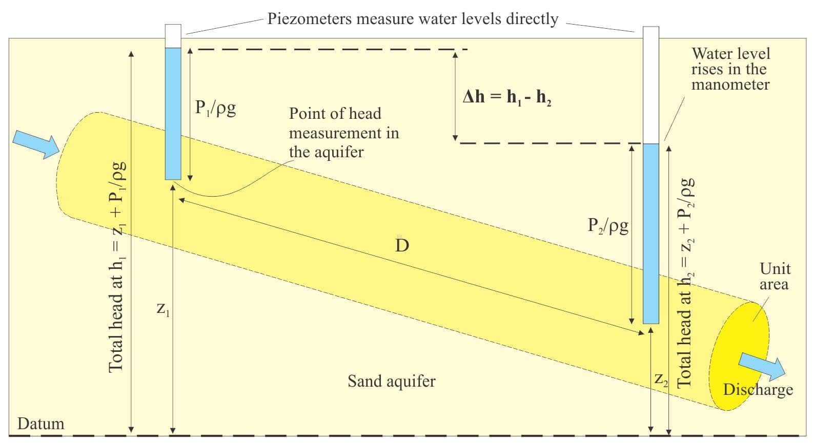
An alternative representation of Darcy’s experiment, shown as tube (pipe) flow in a sand aquifer. Instead of mercury manometers, the piezometers measure the water levels directly, relative to a datum. Each water level represents the total hydraulic head at the point of measurement in the aquifer. The distance D between piezometers allows the calculation of hydraulic gradient.
Darcy’s aquifer was represented by a vertical steel tube, sealed at both ends, with an air-bleed valve at the top. Two mercury manometers were used to measure pressures so that head values top and bottom of the tube could be calculated – the manometers measured atmospheric pressure ± the height of water. Water was added at the top of the tube and discharged from the base.
Darcy and his assistant performed several experimental runs. The tube was filled with water for each run. Sand was added from the top and allowed to settle on the bottom. The thickness of sand was varied systematically (this is D in the above expression), and for each sand thickness the flow rates were also varied. Flow of water into the tube was kept constant for each run; the discharge measured as volume per unit time (the vagaries of water supply at the time meant that keeping flow constant was a bit of a problem). Once steady state conditions had been established in each run, the manometer (pressure) levels were read.
The following graph shows the observed linear relationship between discharge Q and head loss (or head difference) based on Darcy’s data.
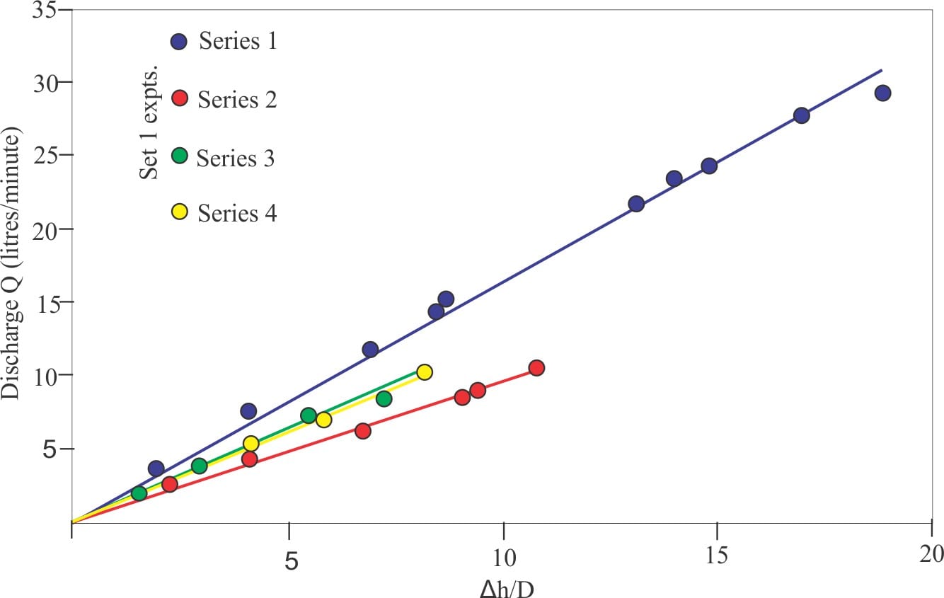
Darcy’s data for Set 1 experiments (there were two sets), replotted as Q versus head gradient for each thickness of sand. Modified from Brown, 2002, Fig. 6.
Darcy’s key observations were:
- Discharge is proportional to the head loss, or head difference along the flow path (Q ∝ Δh), and
- Discharge is inversely proportional to the distance that water travels between the two points of head measurement (Q ∝ 1/D) (in his experiments this is the thickness of sand).
He expressed the proportionalities as: Q = KA (h1 + z1) – (h2 + z2)/D (3)
where Q, K, A, and D as noted above, h is the pressure head, z is the elevation head at the two points of measurement (1 and 2) that are a distance D apart. This is Darcy’s Law. The form of the equation is basically the same as equation (1).
He noted that K varied depending on the sand used (particularly its packing that probably varied slightly for each experiment). We now know that K (hydraulic conductivity) not only varies with differences in the porous medium, but also with the nature of the liquid. Thus, if the sand is the same in two separate experiments, but water is used in one and oil in the other, then the values of K will be different. Later considerations by other workers would establish that K is also a function of dynamic viscosity.
And so…
Darcy’s Law tells us that, under steady state conditions, there must be a hydraulic (head) gradient for flow to occur in an aquifer; in essence it restates the fundamental physical principle that for mechanical work to be done (i.e., to move water from one location to another) there must be an energy potential.
The Law also provides a quantitative solution to determining the parameters for groundwater flow, provided we know something about the porous medium and the fluid itself (that is expressed as hydraulic conductivity). Of course, we can also determine K if we know Q and Δh, and we can measure K experimentally using a permeameter – an instrument that looks similar to Darcy’s original apparatus.
Darcy’s Law describes a flux, and as such is cast in the same mathematical form as Ohm’s Law (current is proportional to voltage), and Fick’s Law (molecular diffusion is proportional to a concentration gradient.
Darcy’s Law is a crucial component of fluid flow modelling, particularly for solving important questions about groundwater, for example the sustainability of aquifers to pumping.
Credits: The historical background to Darcy’s life, his scientific and social contributions were gleaned from Freeze (1994; Brown (2002- open access); and Simmons (2008 – PDF).
Other posts in the Groundwater Series
Whiskey is for drinkin’; water is for fightin!
The Architecture of Connected Holes; A Different Way to Look at the Liquid Earth
“My water well taps into an underground river” and other myths
Coastal aquifers; groundwater at sea
Groundwater contamination; messing around with aquifers
Landslide! How groundwater affects the stability of slopes
GRACE meets LANDSAT; Eyes in the sky monitoring long-terms changes in water resources
A misspent youth serves to illustrate groundwater flow
Contrails, analogies, and visualizing groundwater flow