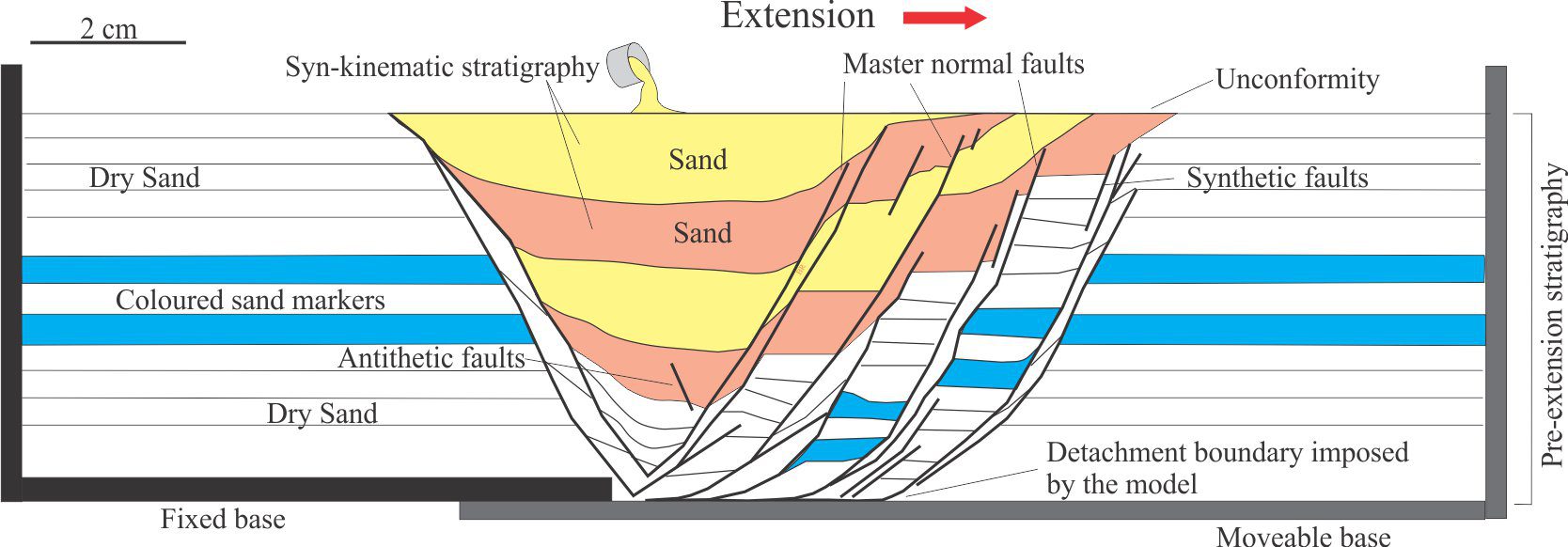
Scaled sand-box experiments are an ideal medium to observe rock deformation that, in this example, involves synkinematic deposition during rift-like crustal extension. The choice of model materials, in addition to imposed boundary conditions such as strain rates, will determine the outcome of the experiment. Dry sand was chosen for this model because its brittle behaviour under the model conditions is a good representation of natural rock failure. Diagram modified slightly from Eisenstadt and Sims, 2005, Figure 3a.
This post deals with the materials, their rheological behaviours, and scaling as they apply to analogue structure models.
Rock deformation
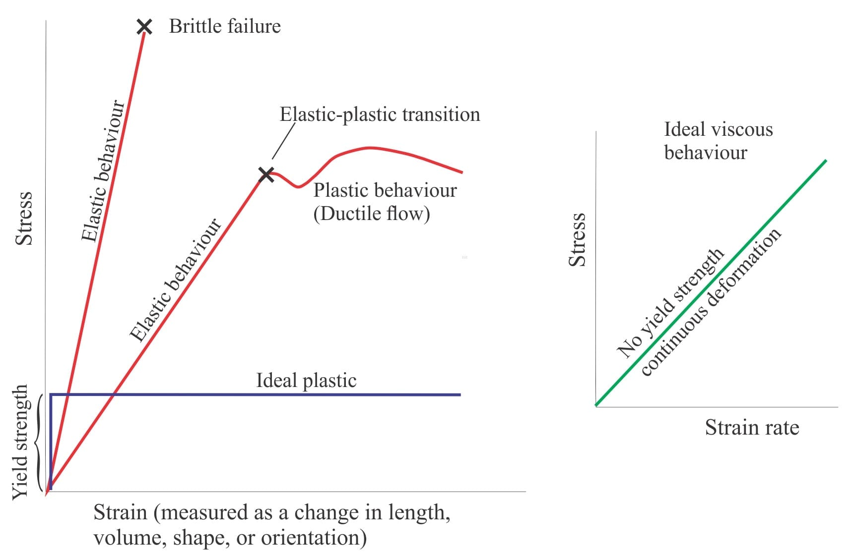
Two of the most common structures generated by rock deformation are faults (and fractures) and folds. The rheological conditions for each are fundamentally different: faults and fractures result from brittle behaviour, whereas folds require materials to act more like plastics with ductile behaviour. Both styles represent deformation conditions beyond the elastic limits of the material involved. For example, hard granite at near surface conditions will exhibit brittle behaviour at high strain rates (confining pressures will be low), but at depth may act in a ductile manner at lower strain rates and high confining pressures (and elevated temperatures). How rocks and sediments behave under stress depends on:
- Lithology and grain/crystal composition and size. The compressive strength of limestone is commonly less than that for quartz arenites because of the propensity for calcite-dolomite crystal cleavage.
- Stress magnitude and orientation. For example, is the principal stress due to lithostatic load, or are there deviatoric and differential stress components?
- Confining pressures – compressive rock strength increases with depth and confining pressure.
- Temperature.
- Viscosity, that depends on lithology, temperature, and strain rate.
- Preexisting anisotropies (fabrics or structures), such as older fracture networks, crystal or grain alignment, metamorphic foliation, and sedimentary stratification.
Rock strength is one measure that accounts for some of these variables; it is a measure of the maximum uniaxial stress at the point of material failure. Failure in this context is usually expressed as a function of the internal cohesion, or cohesive strength, and the internal angle of friction (φ)that for many Earth materials is about 30o to 35o. The SI unit of rock strength is the Pascal (Pa), or megapascal (MPa – dimensions ML-1T-2). Rock strength is defined for tensile and compressional conditions, but for most geological systems where deformation occurs at depth within the crust, compressive strength exceeds tensile strength. Furthermore, the dominant mode of failure is by shear.
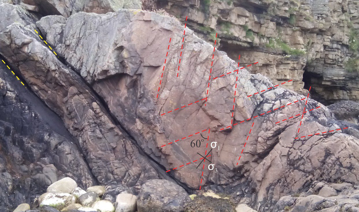
Fracture sets in Old Red Sandstone, Portskerra (north Scotland) – the outcrop face is almost vertical. Red dashed lines follow conjugate fracture sets at a reasonably consistent 60o separation. The dashed yellow lines indicate bedding plane parting that is approximately parallel to σ3 – bedding dips 50o. The point of rock failure in generating these fractures corresponds to the rock peak friction, with a friction angle of 30o (see discussion notes below).
For almost two centuries, analogue modeling of fault (and fold) systems has focused on rifts and inverted rifts, fold – thrust belts and orogenic wedges at convergent plate margins, and strike-slip fault arrays at transcurrent or oblique transcurrent margins. Here are some excellent reviews of analogue models for geodynamic systems (Shellart and Strak, 2016), rifting and salt mobilization (Zwaan and Schreurs, 2022), and orogenic wedges (Graveleau et al., 2012).
What are these structure models attempting to do?
Fundamentally, the models allow us to glimpse processes that under normal geological conditions of time and space we cannot observe. If we scale the model variables correctly, there is a good chance we will answer some of the questions about how these systems operate. For example, the master extensional faults in rift systems are usually accompanied by networks of synthetic and antithetic fault arrays that form at different stages of rifting and sedimentation in fault-bound basins. Analogue models can help us visualize the overall distribution of strain by teasing out the relative timing, orientation, and magnitude of the fault arrays and the displacement of syn-rift stratigraphy. To do this, the model materials need to be appropriately scaled to natural examples.
Material rheology
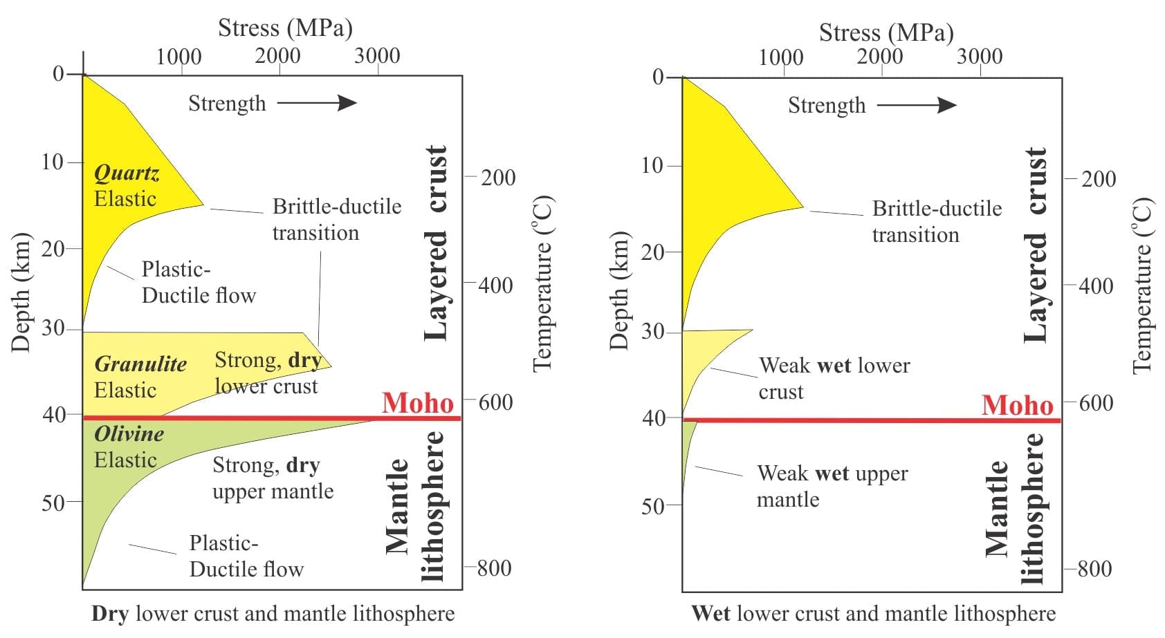
Structure model construction requires materials that are scaled to represent brittle and ductile rheological behaviour, plus behaviours in between these two end-member types. Analogue models built to examine fault initiation and evolution are usually layered – layering can reflect broad stratigraphic ordering of a sedimentary basin, or at larger scales, the layering of lithosphere crust and mantle. The order in which layers of different rheology and thickness are laid down in a model will influence the style of deformation; ductile layers that are prone to folding or flow may affect the distribution of strain in underlying and overlying brittle layers.
The chosen materials must also suit the modeled deformation mechanism. Models that represent diapirism of salt or igneous melts will require viscous materials that flow and have buoyancy contrasts with surrounding rock-material. The reverse buoyancy problem exists for lithosphere-scale models that represent subduction. The energy required to drive these experiments comes from within the models and is manifested as positive or negative buoyancy.
Materials having fundamentally different rheologies are required to model rifted upper crust and synrift sedimentation, where compressive or tensile stresses dominate, and where buoyancy and inertial forces are negligible (although this generalization is complicated where synkinematic salt is deposited). In these experiments, the energy to drive compression-extension originates outside the model, for example, from a worm-screw driven plate at one end of the model container.
Common model materials
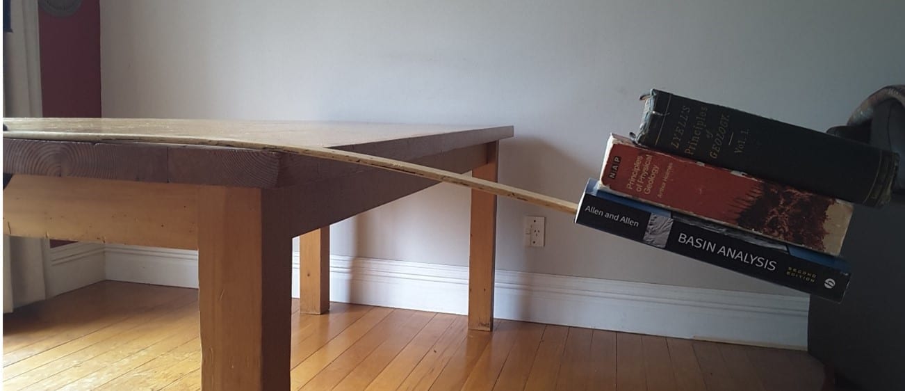
One of James Hall’s first experiments on folding of stratified rock used cloth layers (Hall, 1815). One can imagine Hall at his dinner table, watching the tablecloth deform as plates were moved from diner to diner, and intuiting the analogy with folded rock he had observed in the field. His later experiments used layers of granular and viscous materials, as did many subsequent experimentalists (Caddell, 1889 (see also Butler et al., 2020 ; Willis, 1894; Hubbert, 1934).
Except for the silicon polymers, the materials used by recent experimentalists have changed little from these early pioneering days – the difference is that we now have a good understanding of material properties in relation to their rheological behaviour. Some commonly used materials and their properties include:
- Well sorted, dry, quartz and feldspar sands (brittle behaviour, low cohesion). Bulk densities range from 1.56 g.cm-3 (quartz sand) to 1.3 g.cm-3 (feldspar) (bulk density is less than the mineral density). Mean peak friction coefficients are 0.5 – 0.6 and friction angles are 31o-36o. Some studies have assumed that dry sand is cohesionless, but repeated lab analyses show that mean peak cohesion ranges from 10-140 Pa.
- Corundum/magnetite sands, commonly used as marker layers (brittle behaviour). Bulk density about 3.3 g.cm-3.
- Wet clay – also used for brittle failure and has cohesive strength slightly higher than dry sand (Eisenstadt and Sims, 2005). Density depends on water content – commonly ~1.6 – 1.8 g.cm-3. Peak cohesion up to 100 Pa.
- Kinetic sand (adding a touch of viscosity with 1% -2% silicon polymers). Either quartz or corundum mixtures. Viscosity varies with density (% polymer) and ranges from about 4 x 10⁴ to 105 Pa.s
- Gelatins (visco-elastic to brittle rheology in the gel state depending on strain rates and confining pressures) (Kavanagh et al., 2013)
- Silicone putty (a viscous polymer representing ductile behaviour). Viscosity 104 to 105s.
- PDMS (polydimethylsiloxane) – a more fluid silicone polymer. Density 0.98 cm-3 and a viscosity around 1.6 x 10⁴ Pa.s.
- Syrup (sugar, honey – low viscosity ductile flow). Viscosities <1 to 20 Pa.s.
Material properties
Faulting in the brittle upper crust generally obeys the Coulomb criterion for failure and frictional sliding, and is written as:
τ = C0 + Tanφ σN where τ is the shear stress at the point of failure, C0 is the rock cohesive strength, φ is the internal friction angle, and σN is the normal stress.
The same empirical relationship should also hold for models and model materials (to be consistent with the rules of similarity). The Coulomb function emphasizes the variables we need to scale such that the ratios between model variables and natural variables are similar – for example, C0 model/ C0 real ≈ Lengthmodel/ Lengthnatural.
Model variables that map brittle behaviour
Tan φ: This is the friction factor, or friction coefficient – it is dimensionless, usually written as
τ = C0 + γσN where, for rock materials, γ is the coefficient of internal friction and is the ratio of the frictional force to normal force – it depends primarily on surface roughness. Thus, γ is zero for a frictionless, smooth, or lubricated surface. For most rock materials γ is 0.6 – 0.7. The presence of clays, or mica-lined schistose foliation will tend to lower the values of γ.
C0 – Cohesion (Cohesive strength): (Dimensions ML-1T-2). C0 is a function of material density, the acceleration due to gravity, and a length dimension. Bulk densities are well within an order of magnitude of real rock densities, the gravitation constant is the same for model and the real world, and lengths commonly scale from 10-4 to 10-6 (at 10-6 one cm scales to 10 km). If the Coulomb criterion is to apply to the models, then the cohesive strength must also scale to 10-4 to 10-6.
φ – friction angle: (dimensionless). A good analogy for representation of the internal friction angle (φ) is the angle of repose for dry, well-sorted sand; the actual value is about 34o. If the slope increases it becomes gravitationally unstable and grains will slide or tumble downslope until the repose angle is re-established – in other words, the granular material shears. This basically is the model applied to failure of harder rock where shear is caused by differential normal stresses.
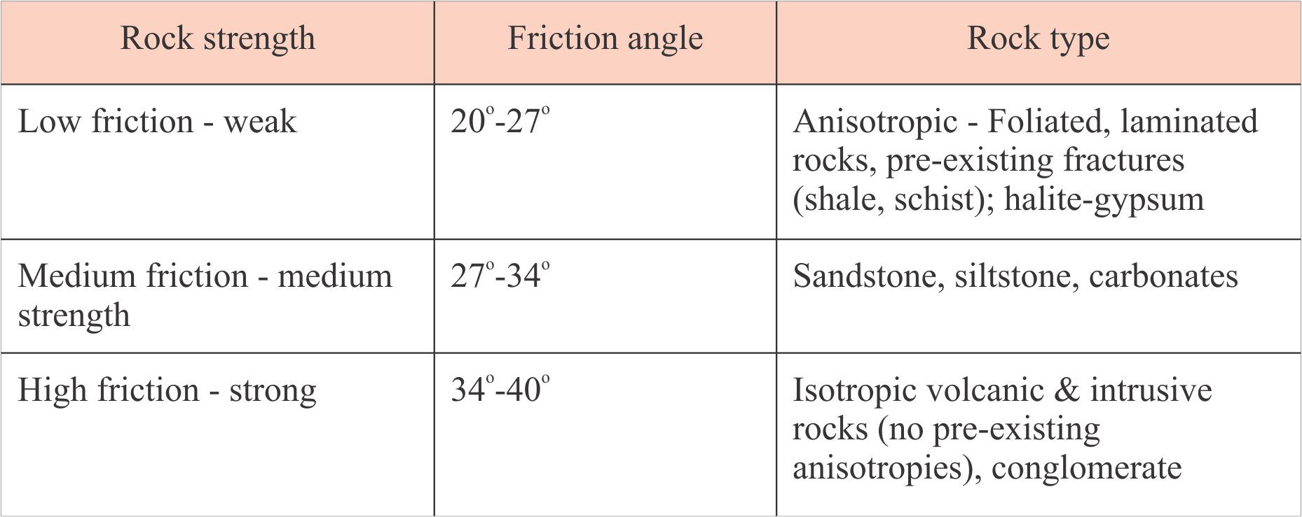
Friction angles for different rock types and rock strengths, from Wyllie and Norrish, 1996. Table 14-1.
Viscosity – mapping ductile behaviour
This is one of the fundamental measures for materials where ductile behaviour is important. Viscosity is dependent on temperature and strain rate, and testing is done at specified values of these variables. Silicone putty is commonly used in fault models to represent shale or salt that are inter layered with brittle lithologies. It is also used as a basal layer of models that represent salt flow or more ductile behaviour deeper in the crust and mantle lithosphere.
Kinetic sand is a mixture of either quartz or corundum/magnetite sand and about 2% silicone polymer (polydimethylsiloxane, or PDMS). The polymer adds a degree of cohesion and viscosity to the mix, that represents rheological behaviour somewhere between brittle and ductile. PDMS has a density of 0.98 g/cm3, its viscosity averages 3×10⁴ Pa.s at 23 °C (Konstantinovskaya et al., 2007). PDMS can also be used on its own to represent salt layers (e.g, Ferrer et al., 2023) or ductile mantle lithosphere. An example of the PDMS viscosity- shear rate relationship is illustrated below.
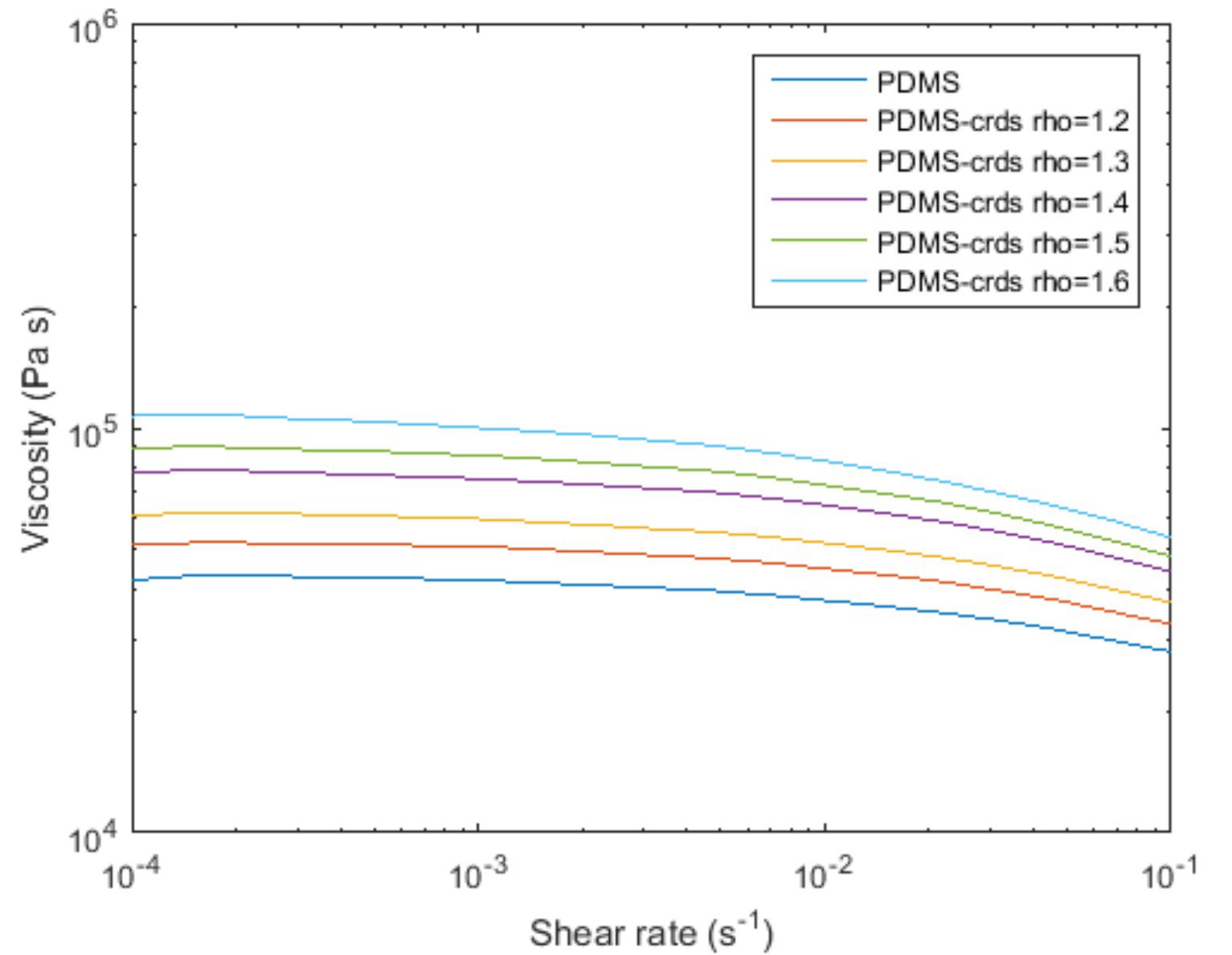
Lab test plots of viscosity – shear rate for corundum sand – PDMS mixtures at different densities – pure PDMS density is 0.98 g/cm3 (top curve). From Zwaan et al., 2018, Figure 1.
Silicone putty (a kind of Silly Putty) is also a viscoelastic silicon polymer that has unique properties in that it reacts elastically if the strain rate is high (e.g., bouncing it off the floor), and as a viscous fluid at much lower strain rates. The latter property makes it ideal for models of deformation involving ductile behaviour. Some of the strain in the deformation models is taken up by folding of the ductile layers. It has a viscosity of about 4×10⁵ Pa.s at 23 °C depending on composition (a bit higher than PDMS). At the experimental strain rates of most models, silicone putty behaves as a Newtonian fluid (i.e., it has no inherent strength and begins to deform immediately stress is applied). Newtonian properties are important in analogue modeling because the behaviour of the materials doesn’t change during the experiment.
Sugar syrups are also used in lithosphere-scale models to represents the asthenosphere-lithosphere boundary. Syrup is also used in experiments where isostatic compensation is modeled (Schmid et al., 2022). Average measured viscosity, depending on composition, ranges from about 7 Pa to 64 Pa.s
Material scaling
The average values for C0, m, and γ for granular materials used in the models have been determined from repeated lab determinations. Both the friction coefficient and cohesion have measured values that record peak stress conditions at the point of failure – these are recorded as peak cohesion (peak cohesive strength) and peak friction respectively. Dynamic cohesion and dynamic friction represent the plateau on the shear stress curves, that reflect the forces opposing continued motion along a fracture plane; their values are generally lower than those for peak conditions. The example below of shear stress-strain illustrates this relationship.
The average lab determined peak friction coefficients (dimensionless) for quartz sands are about 0.6 – 0.7, which is consistent with measured rock values.
Internal friction angles for the sands are commonly 27o-35o, also consistent with natural rock values.
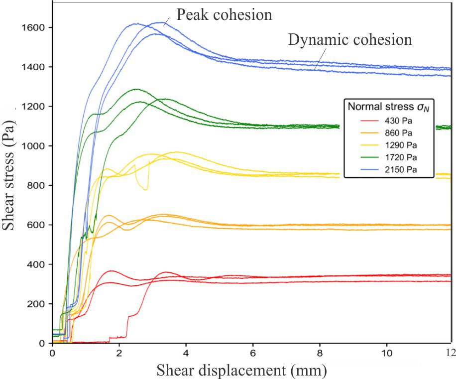
Lab test results for determining cohesive strength and friction coefficient for quartz sand, at different normal stress values (Pa). The peak and dynamic domains for each quantity are well defined. Note that shear displacement has the same dimensions as strain (L). Modified from Zwaan et al., 2018, Figure 2.
Cohesive strengths for most granular materials used in these models range from about 50 Pa to 200 Pa, depending on mean grain size and standard deviation (sorting), and to some extent on the variability of grain shape in natural sands – the use of microspheres can reduce this type of uncertainty. In contrast, the cohesive strength for Earth materials ranges widely from less than 0.1 MPa for soft soils, to >200 MPa for rocks like isotropic granite, marble, and basalt. The range for sandstones is about 50-100 MPa, and < 25 MPa for chalk and salt. If we assume an average value of 60 MPa for sandstones, and 60 Pa for sands used in the models, then the scale ratio is 10-6, which is consistent with the upper end of our length scale.
Viscosity scaling is less obvious, because the scaling factor between ductile materials like silicone putty or PDMS (viscosities in the range 104 to 105 Pa.s) and the average crustal rocks (1018 – 1020 Pa.s) is 10-14 to 10-16. This is hugely different to the 10-5 – 10-6 commonly used for the other scaled variables.
[Scaling factor is the ratio between model variable and natural variable, and hence is dimensionless). It is usually indicated by an asterisk. Dimensionless quantities established for natural systems can be applied directly to analogue models.]
We can solve this apparent dilemma by going back to basic Newtonian mechanics. Newton was the first to demonstrate the empirical relationship between shear stress and the rate of shear deformation, or strain rate, in a fluid. This is expressed as:
τ = μ (v/d) where
τ is shear stress, μ is dynamic viscosity, v is velocity and d a length such that v/d is the velocity gradient for shear, also called the strain rate (dimensions of T-1). If the relationship between stress and strain rate is linear, then the fluid is Newtonian. Under the experimental conditions for most analogue models, materials like silicone polymers behave as Newtonian fluids.
We can rearrange this function for viscosity (μ = τ/ (v/d)) and write dimensionless quantities for its variables using scaling factors – a model/natural stress scaling factor (τ *) and a model/natural strain-rate scaling factor ((v/d)*) and compare the ratio between these two factors and a viscosity scaling factor (i.e., viscositymodel/viscositynatural, or μ*). If the stress factor – strain rate factor ratio equals the viscosity factor, and d is scaled according to other variables in the model, then viscosity is considered to be scaled appropriately (i.e., μ* = τ */(v/d)*). Most modellers who employ ductile materials in their experiments use this method to check the scaling for viscosity (e.g., Davy and Cobbold, 1991; Caniven and Dominguez, 2021; Zwaan et al., 2022.
Afterword
Accounting for variable scaling is an essential part of analogue modeling – get the scaling correct increase the chances of producing model results that mean something, that answer fundamental questions about processes. However, the choice and scaling of model materials doesn’t necessarily ensure model success. Other imposed boundary conditions influence the result:
- The geometry of the model container, particularly its moving parts that drive extension, compression, translation.
- The rates of processes like deformation, sedimentation, or base-level change imposed on the model; should rates be linear or variable?
- Accounting for temperature and geothermal gradients in analogue models is notoriously difficult, and yet for many crustal processes these variables are fundamental. For example, oceanic and continental rifts are commonly accompanied by volcanism and high heat flow. Can we find model materials that are compatible with such conditions where rock viscosity and cohesive strength are scaled appropriately?
Is there value in combining analogue modeling with numerical modeling to help solve some of these problems? At its heart, modeling is a creative scientific exercise that can lead us in unforeseen directions of discovery. Charles Lyell’s dictum The present is the key to the past is an invitation to recreate that past using all the tools at our disposal including using analogue, numerical, and conceptual models. We should continue to RSVP and accept the invitation.
Other posts in the series on geological models
Geological models: An introduction
Model dimensions and dimensional analysis