Tag Archives: scicomm

Kinematic analysis of deformed rock

This post is part of the How To… series

Kinematics is the branch of classical mechanics that studies movement. Questions of movement in the geological world center on deformed rock, the kind that produces fault zones and landslides, thrust sheets and folds, or entire mountain belts and the evolving boundaries of tectonic plates. Our analyses can probe single crystals in thin section, or entire mountains.

Kinematic analysis is essentially a geometric exercise. In the geological world, kinematics is concerned with the change in location (translation) of a body of rock or parts of a rock, its rotation, distortion (changing shape), and dilation (changing size). Changes in location and orientation are described as rigid body deformation; in this case the body of rock is unchanged apart from wholesale movement. Deformation that results in a change in shape or size of a rock body is referred to as non-rigid. Note that there is no reference to the forces that bring about deformation.

In the diagram above I have overlaid the image of a cobble (hard andesite) with an orthogonal grid. The grid provides useful reference points for changes in position or shape. In the case of translation via faulting, we can measure the separation of two reference points to determine the amount of displacement. Rigid body rotation can be measured as an angular displacement with reference to clockwise/counter clockwise movement (in this case it is important to record the direction of observation). Distortion and dilation can be measured as changes in lengths, for example changes in the major and minor axes of the cobble will indicate the degree of shortening or stretching. In this case, assumptions need to be made about original shape and this is where body fossils, some trace fossils, and objects like ooids are particularly useful because their shapes are well known.

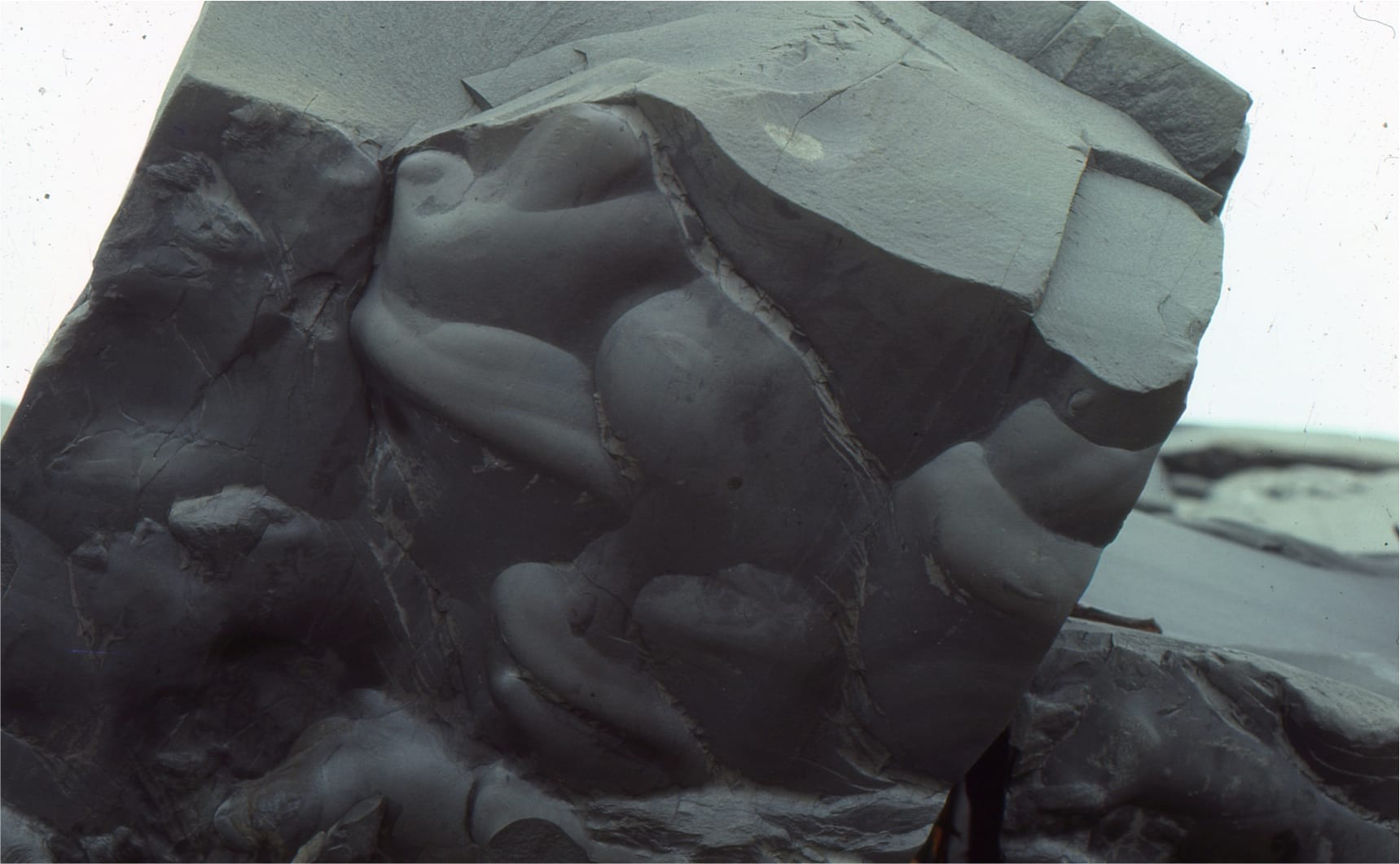
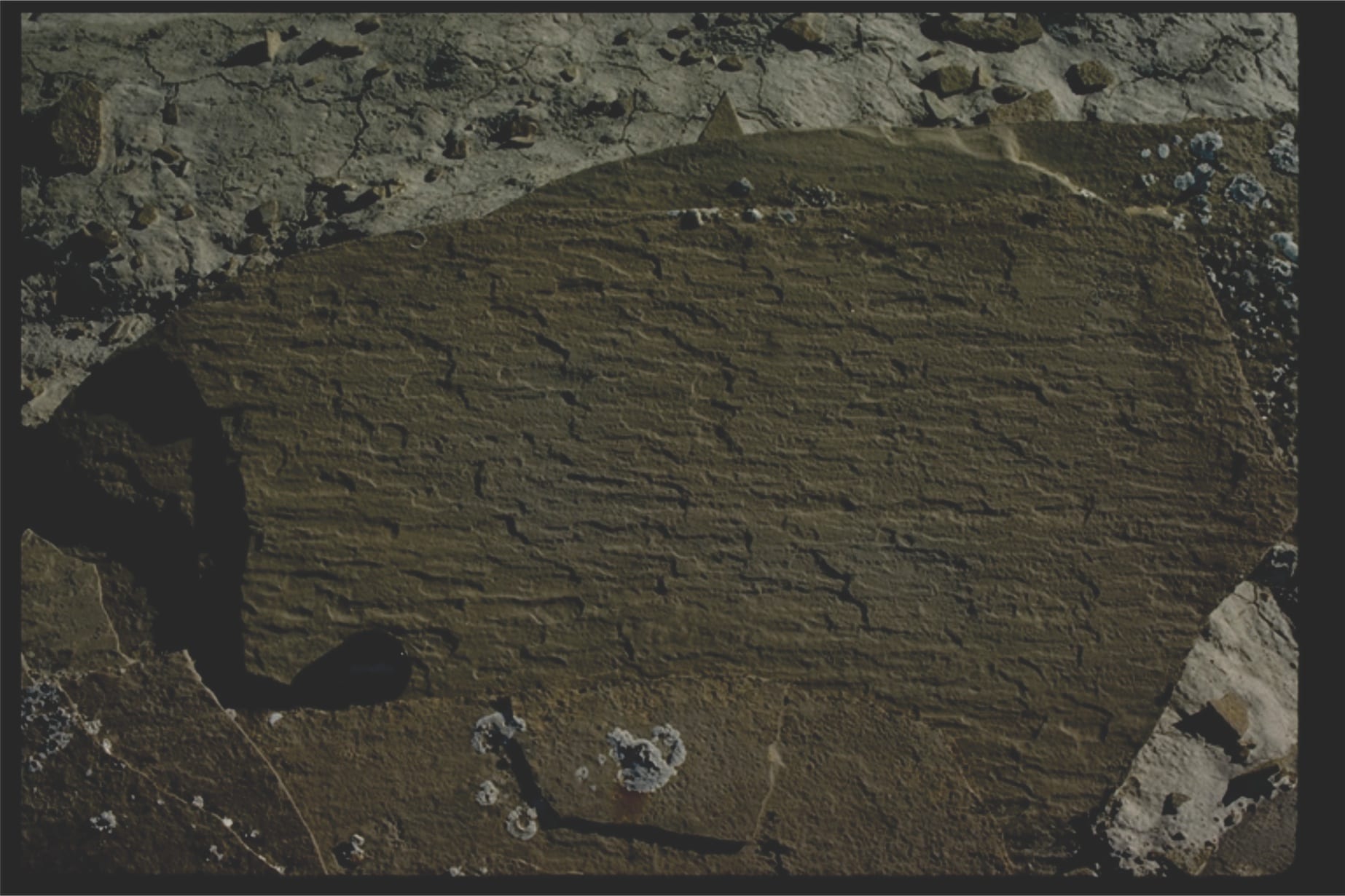
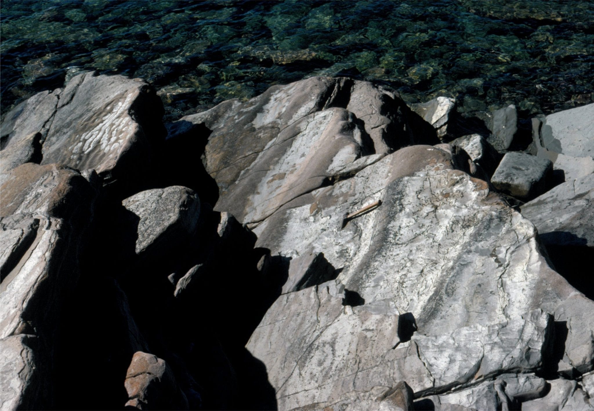
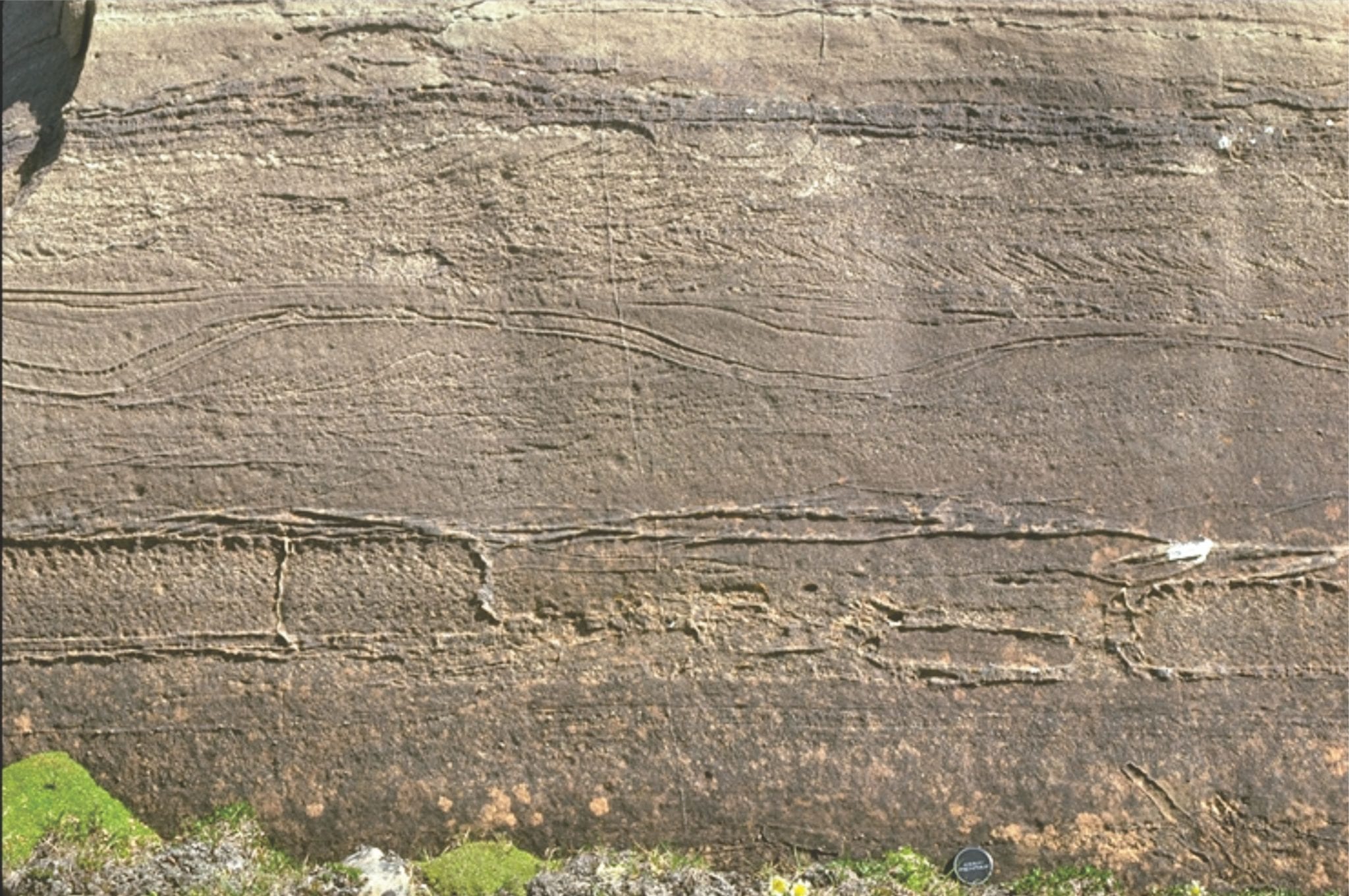
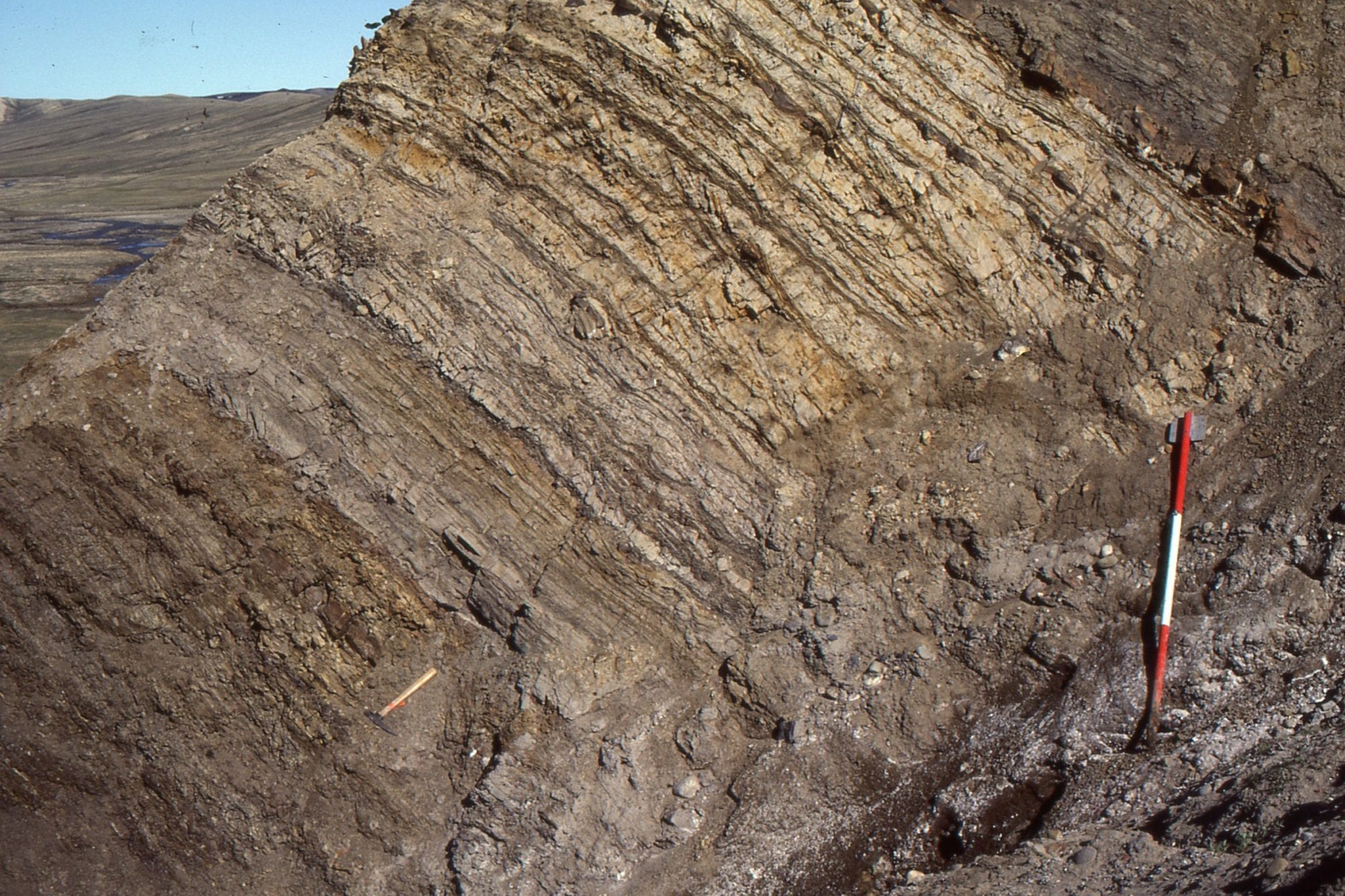
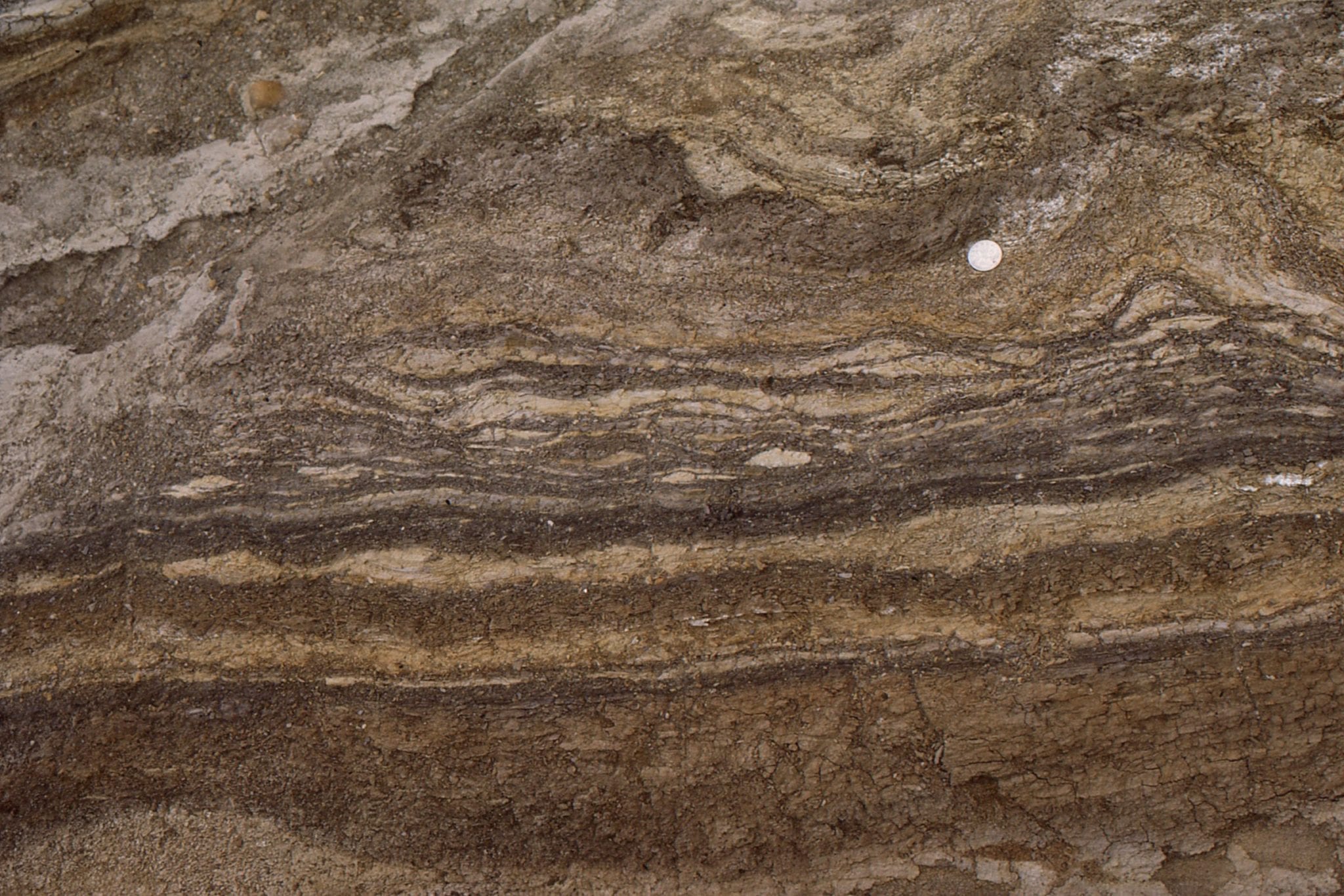
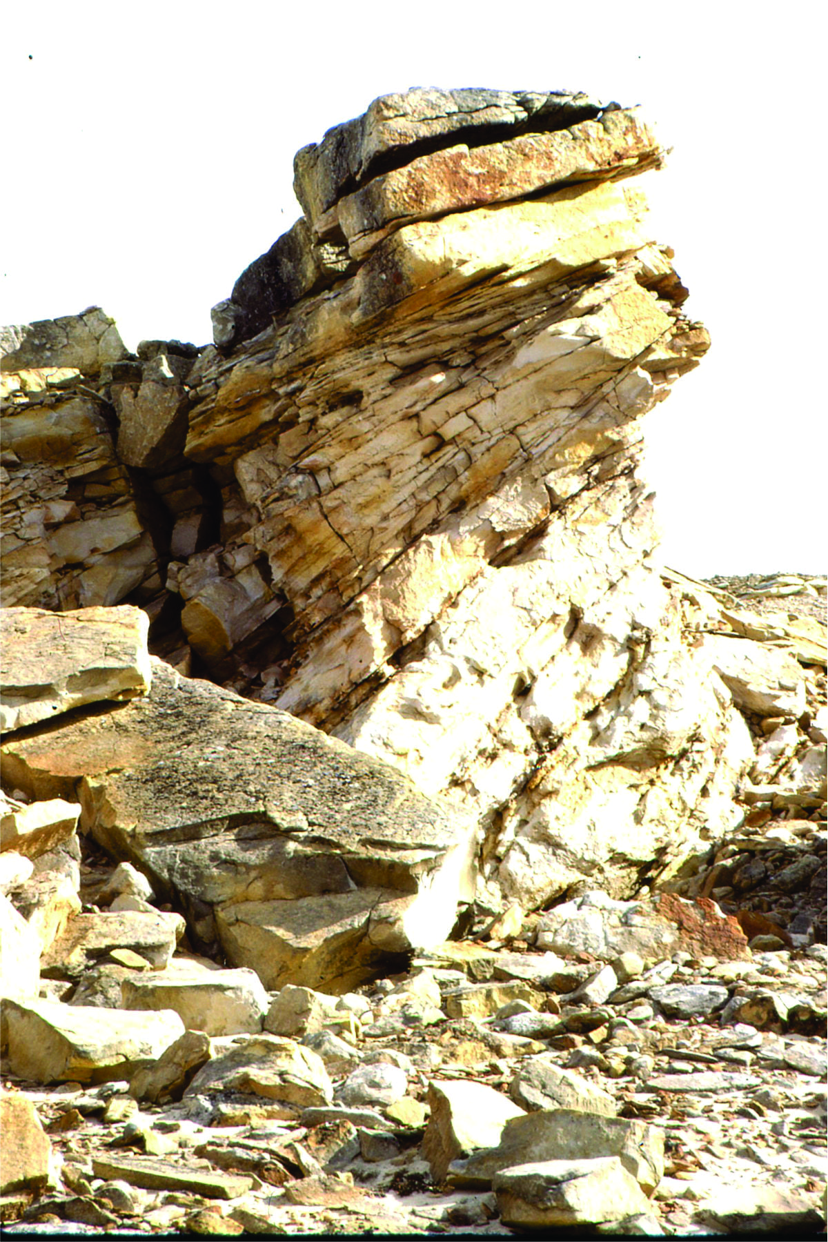
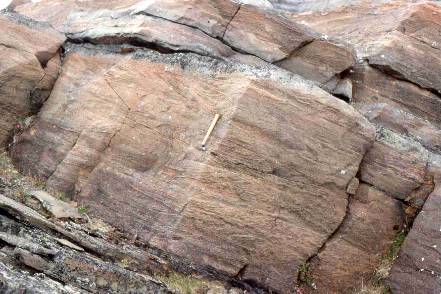
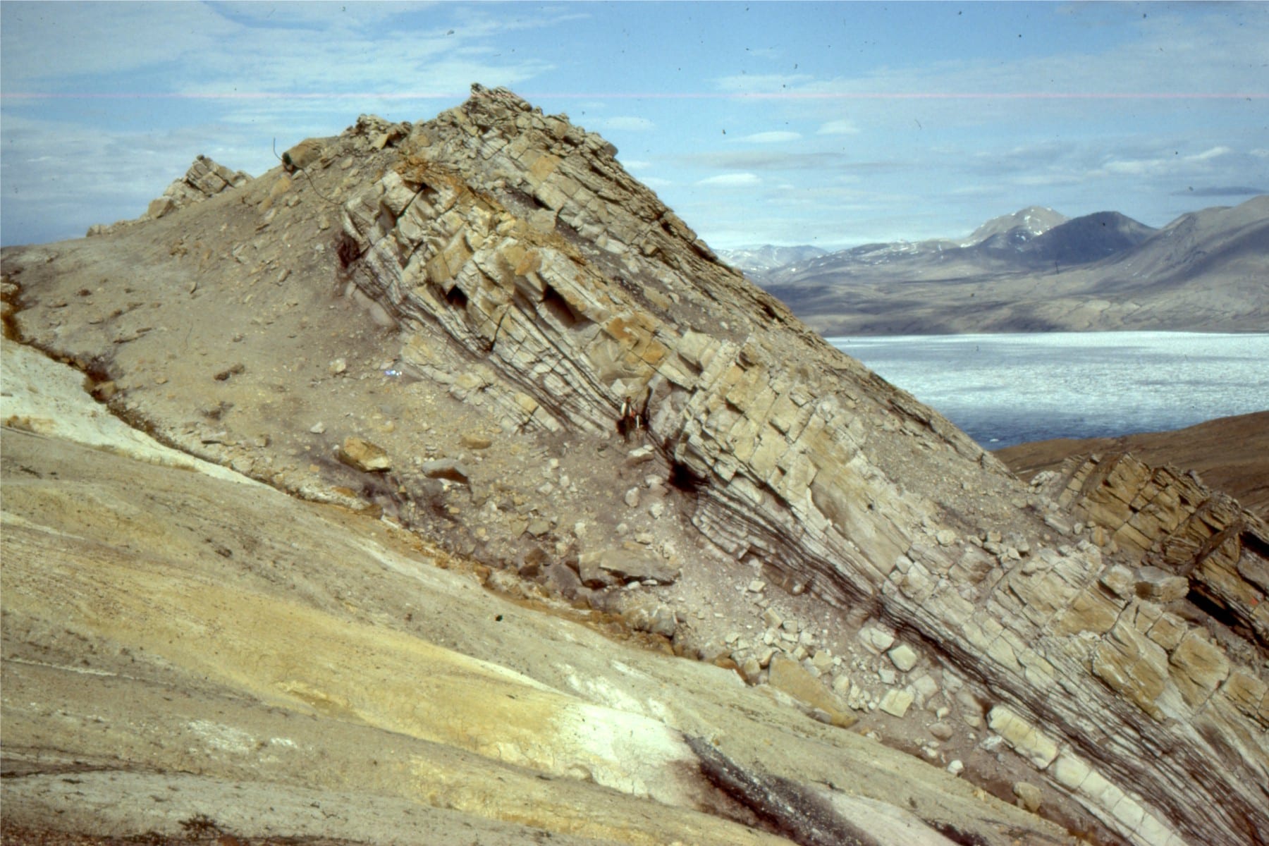
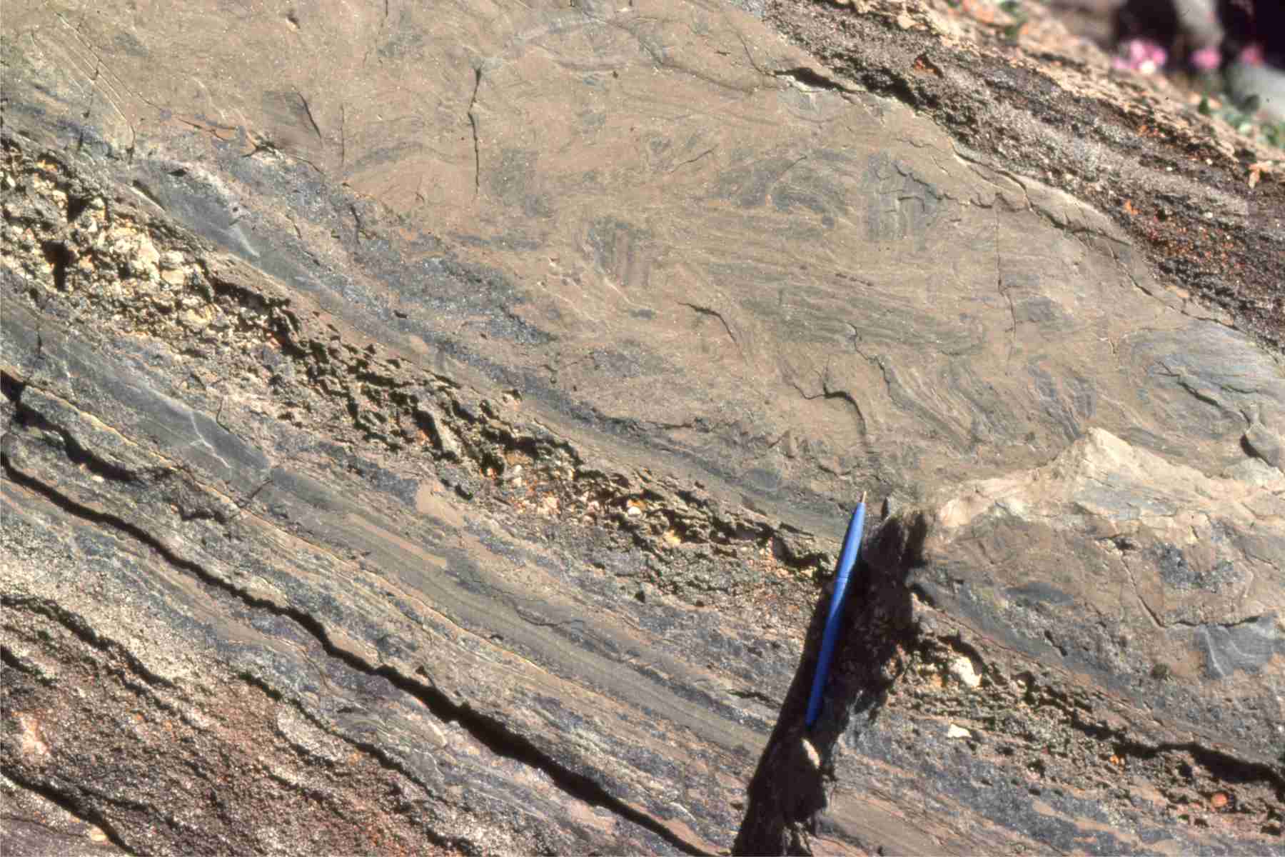
The four end-member conditions are a useful starting point for kinematic analysis but deformation of rock commonly creates more than one geometric response. Boudinage is the extension of contiguous rock into separate blocks (translation); if there is a component of shear these blocks will rotate. The example from Belcher Islands illustrates this nicely – each sandstone boudin has been rotated as a rigid body. However, the surrounding shale has behaved in a more ductile manner and became distorted as it filled gaps between the boudins.

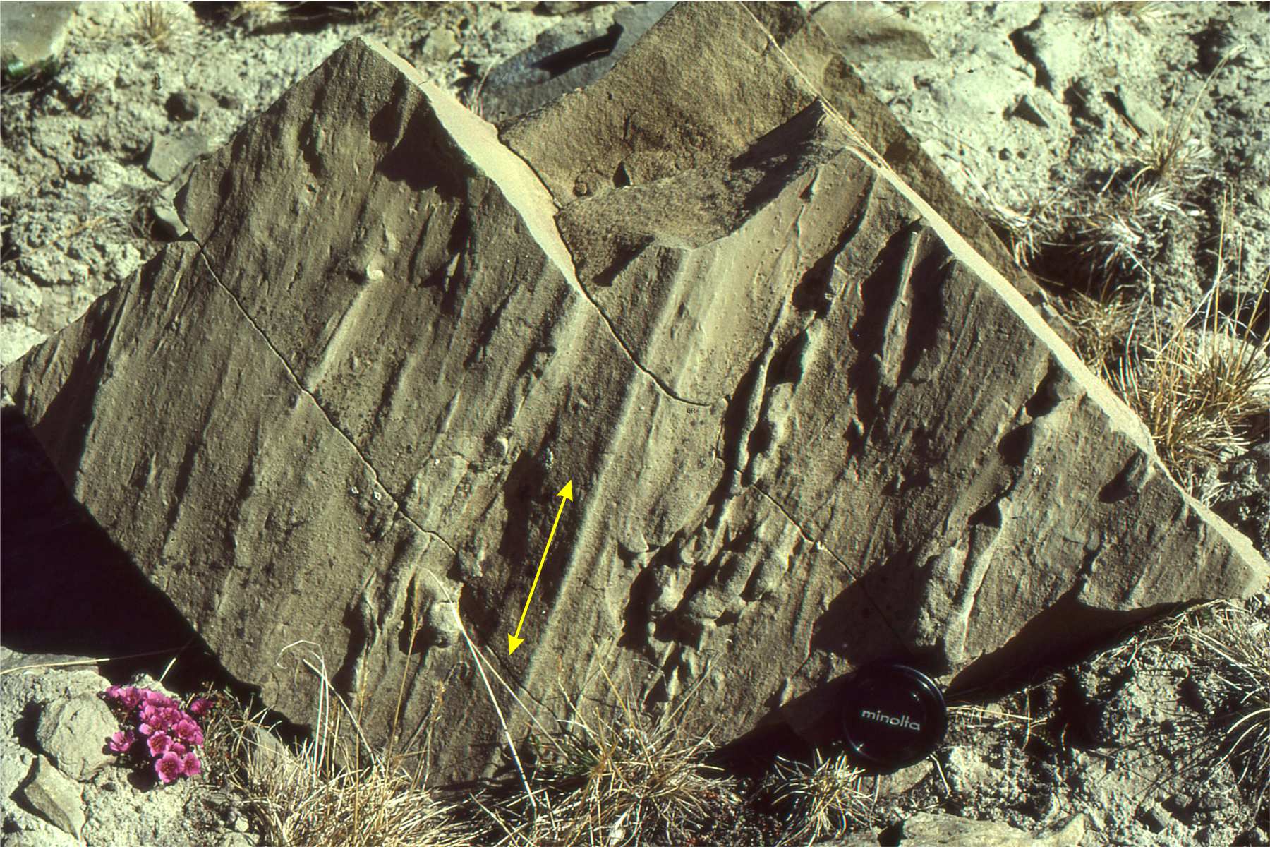
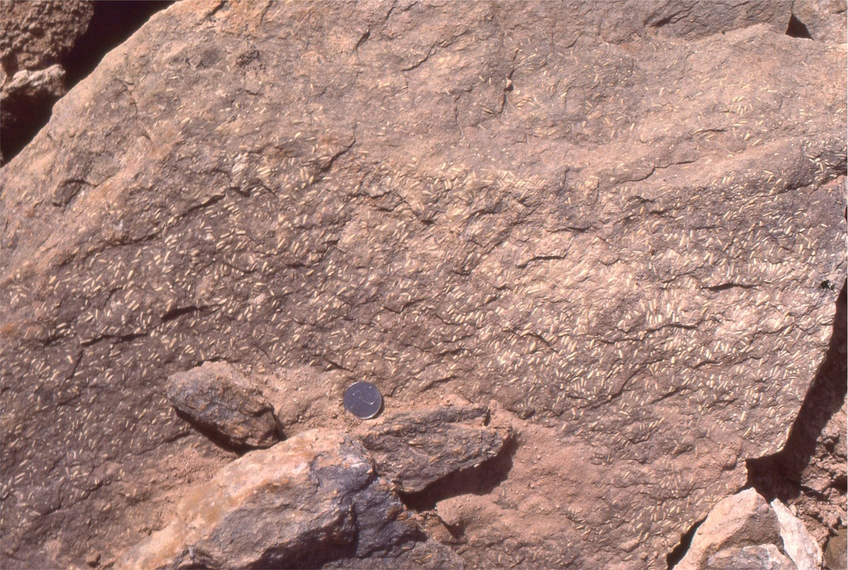
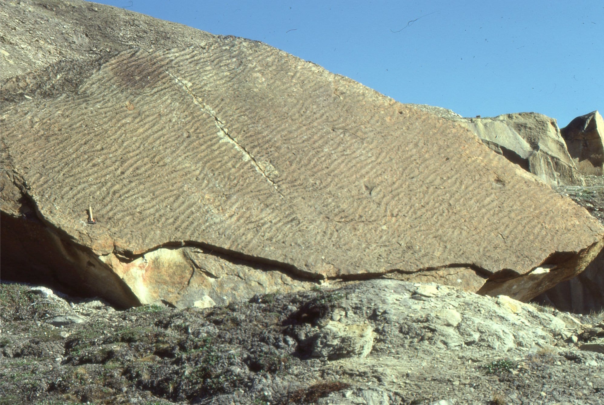
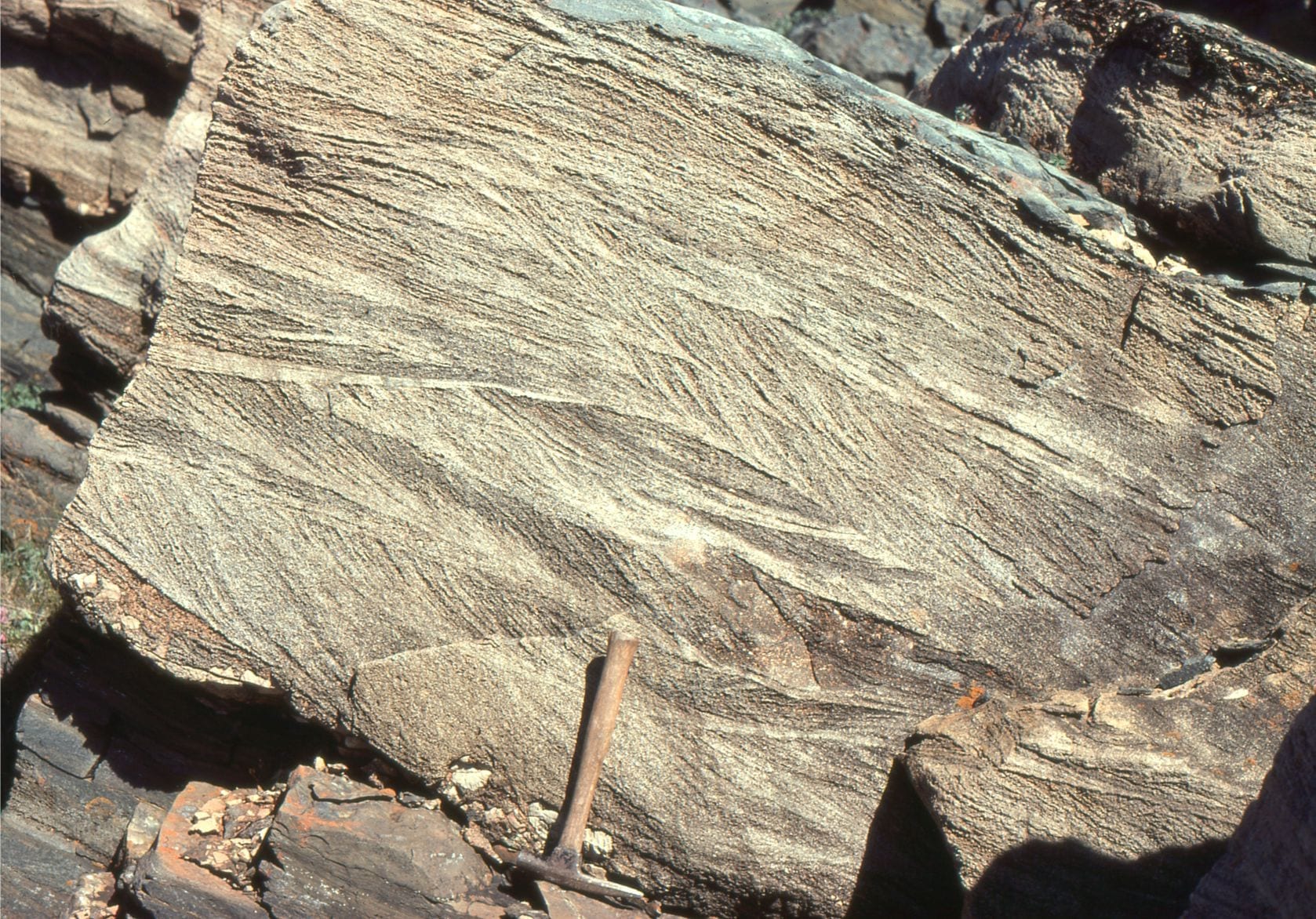
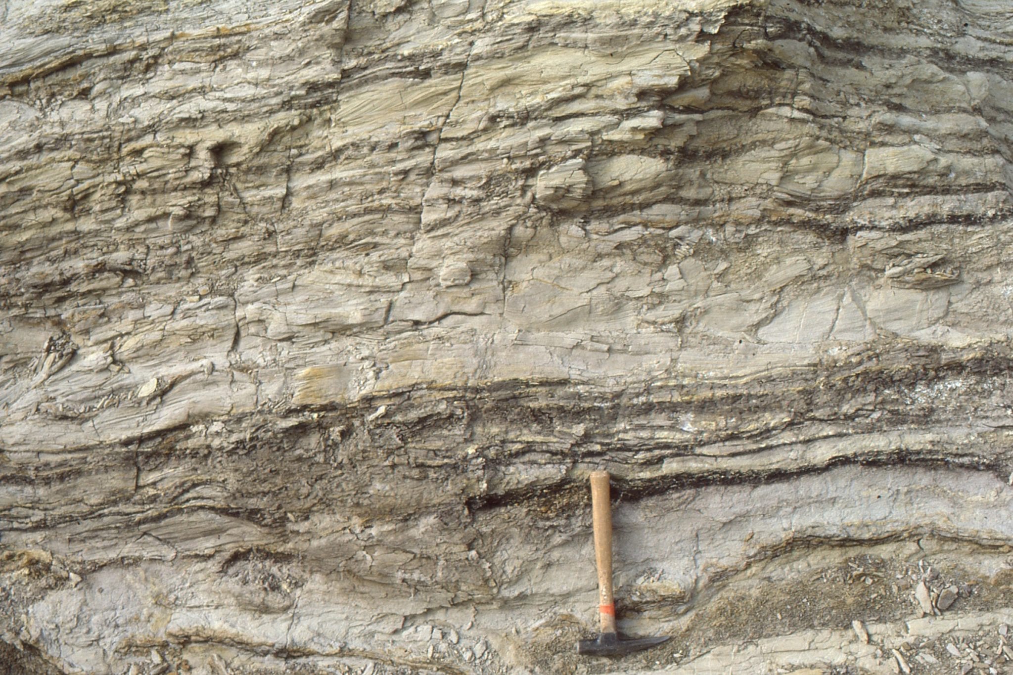
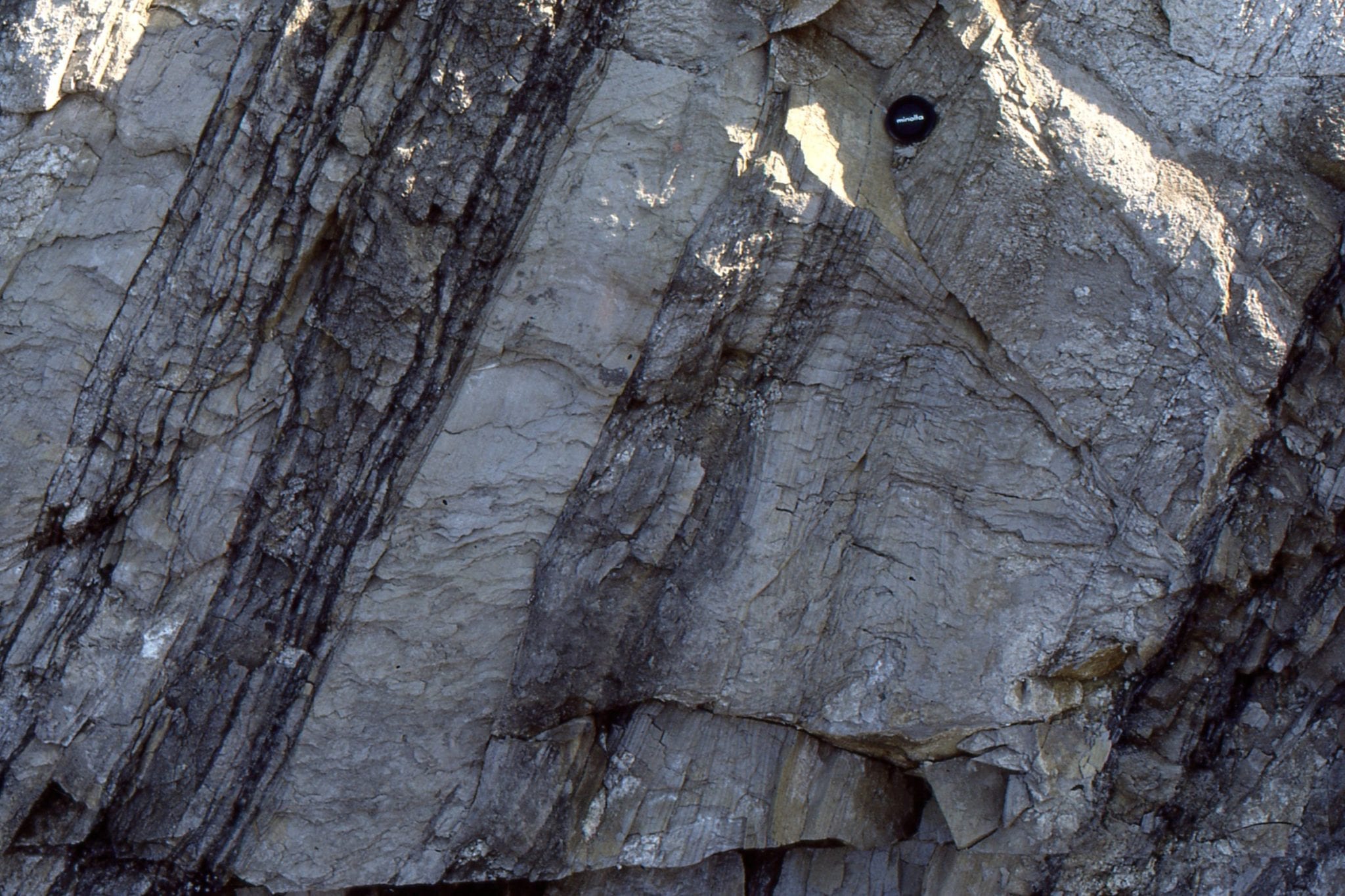
More extreme examples of stretching are shown in the example of an Archean conglomerate from two outcrops near Tamiskaming, Ontario. In this case we don’t know the original shape of the clasts, but we can get a sense of the change in shape (stretching) between the two outcrops. In both examples the clasts have acted as non-rigid ductile bodies.

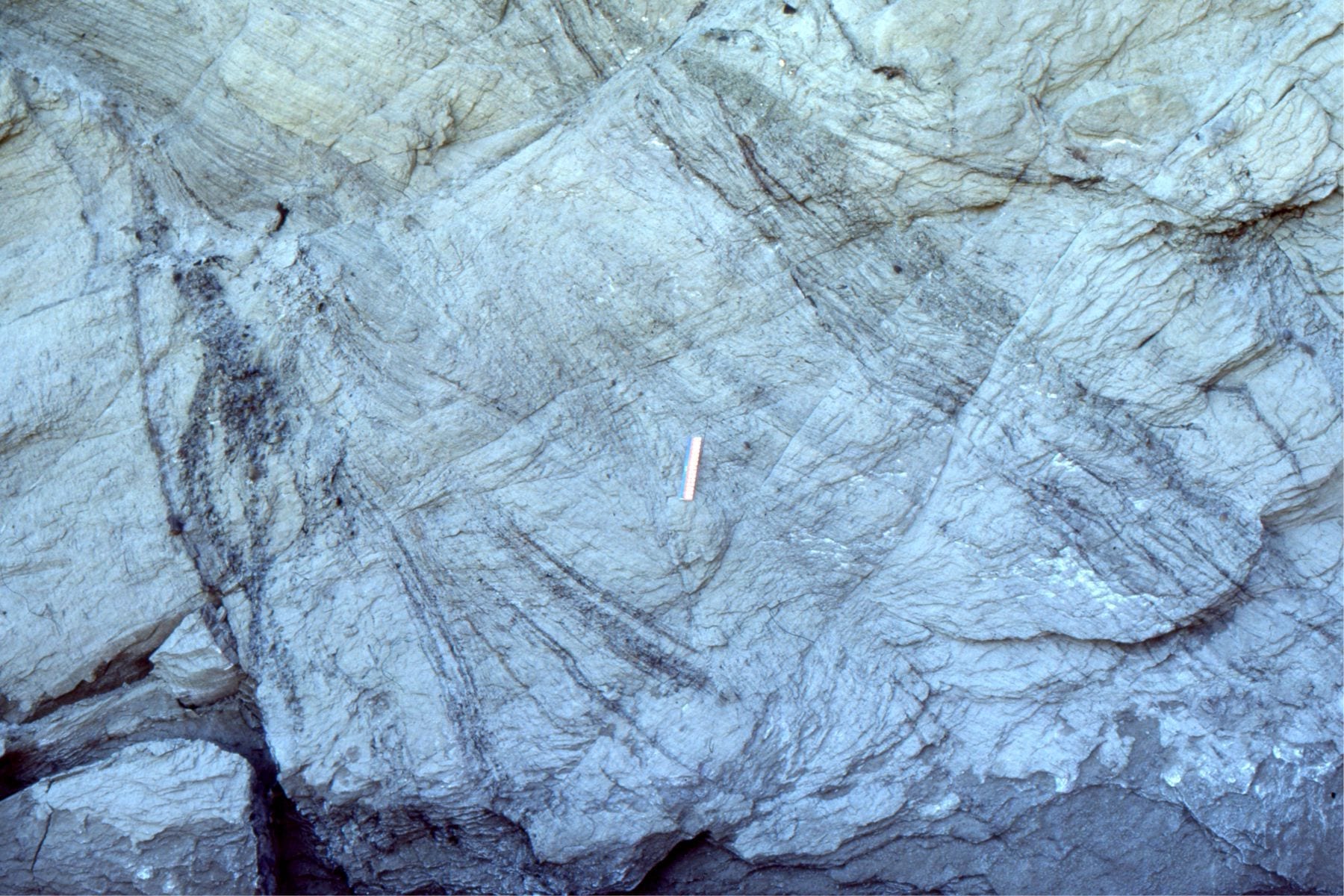
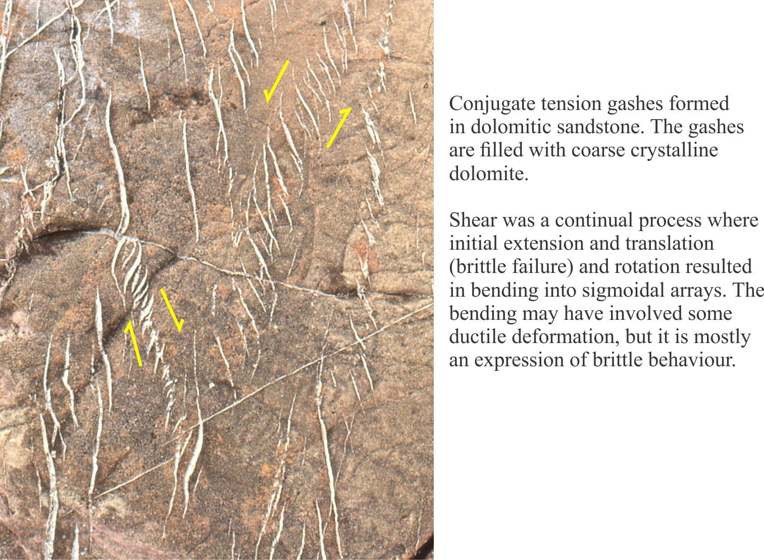
Tension gashes, common in fault zones, also provide a nice illustration of translation (initial rigid body extension), followed by rotation and, if shear continues, distortion. The result is a set of en echelon, sigmoidal gashes that are eventually filled by crystalline quartz or calcite/dolomite. The crystal precipitates may also exhibit some degree of deformation.

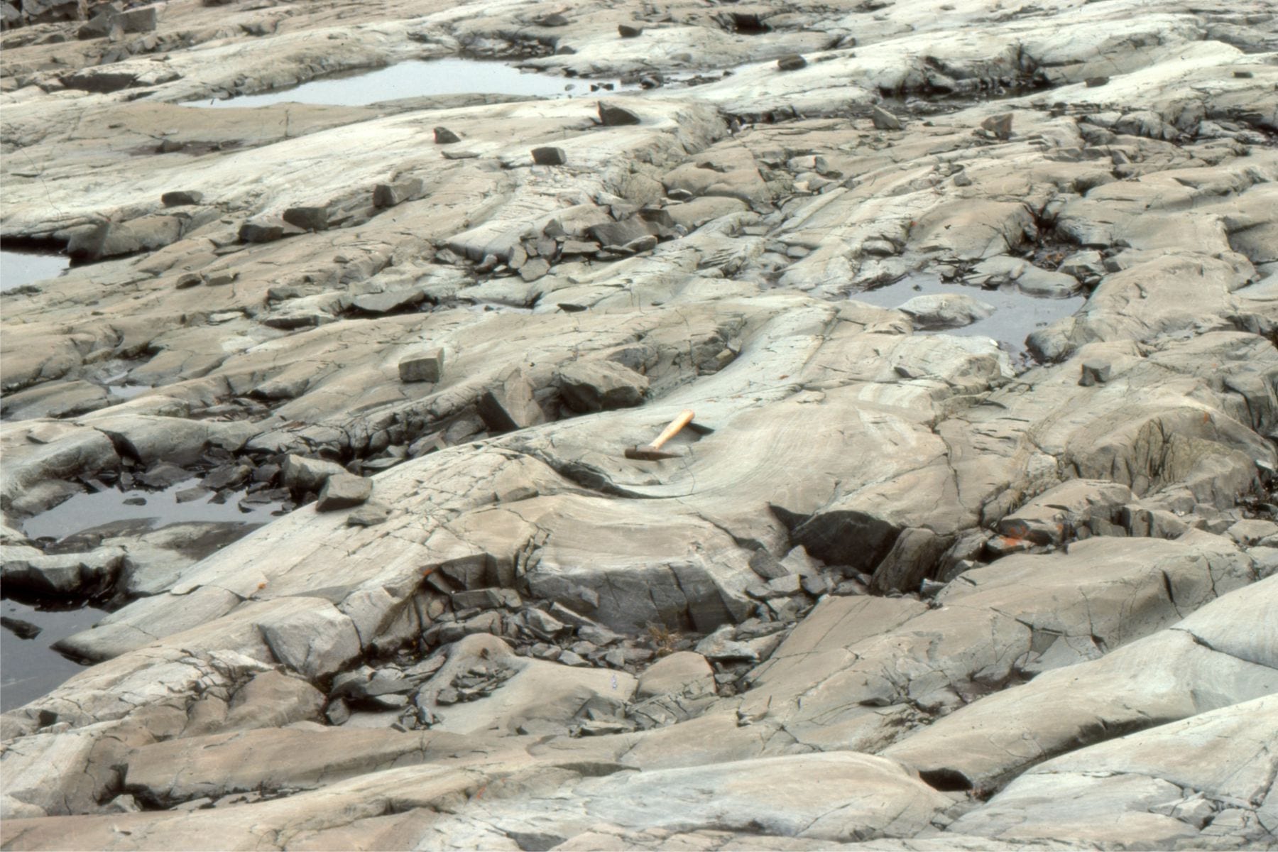
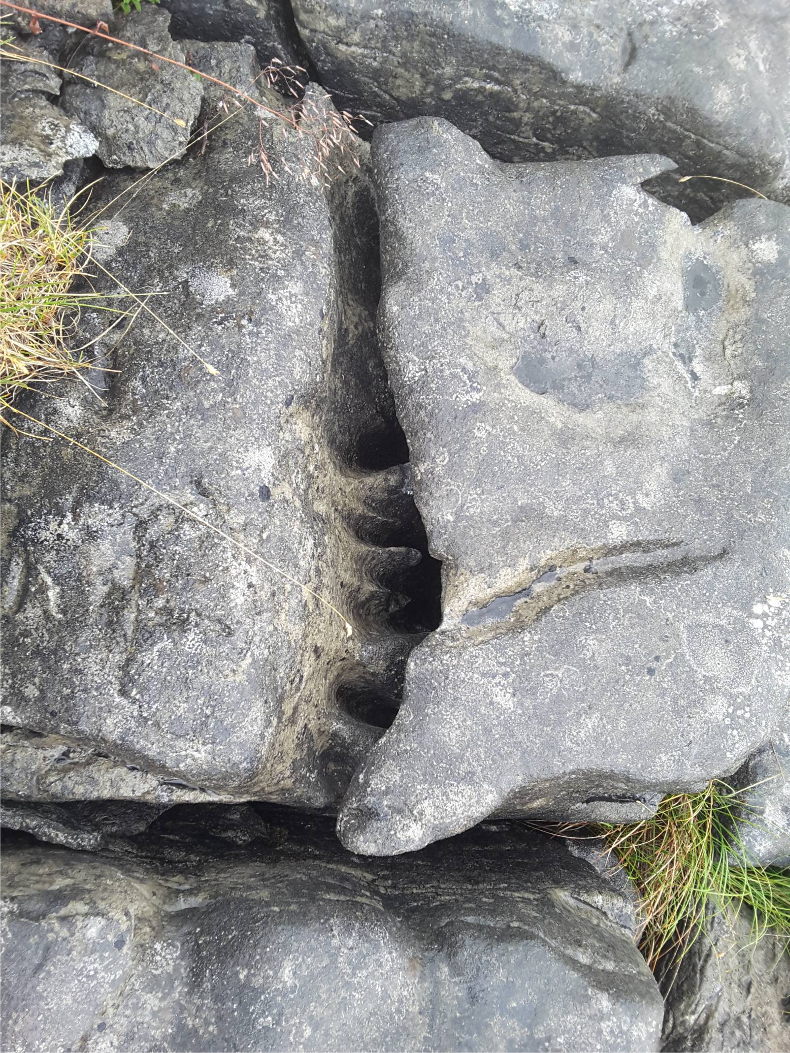
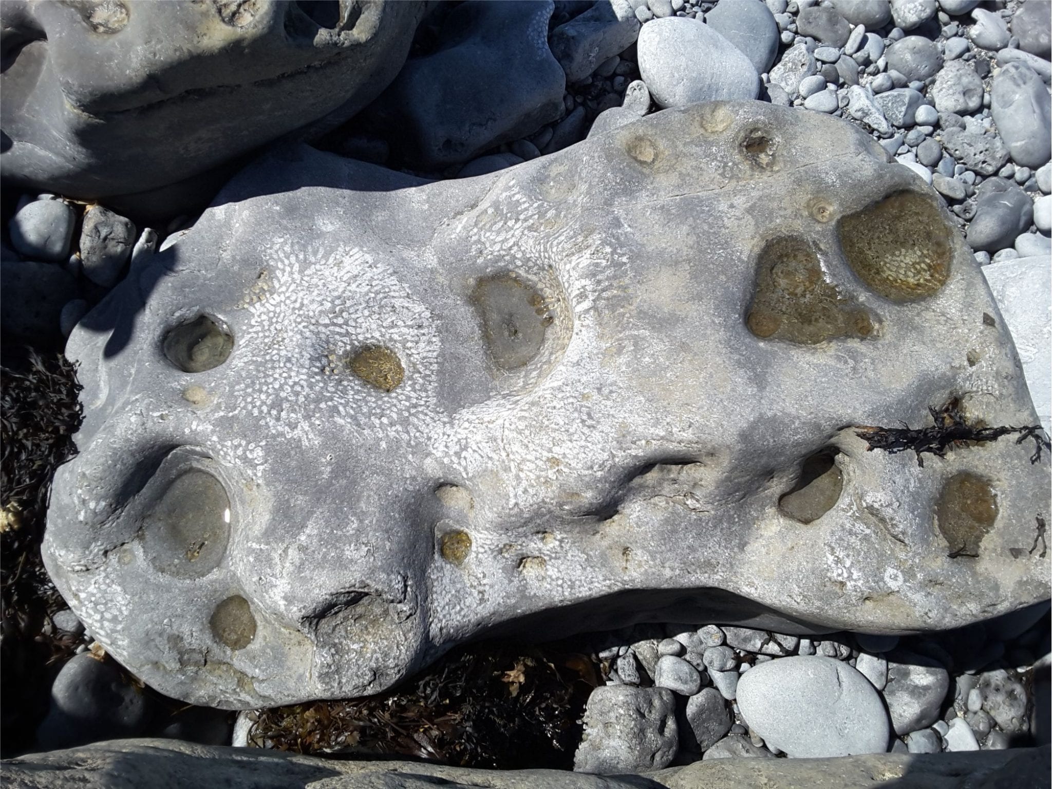
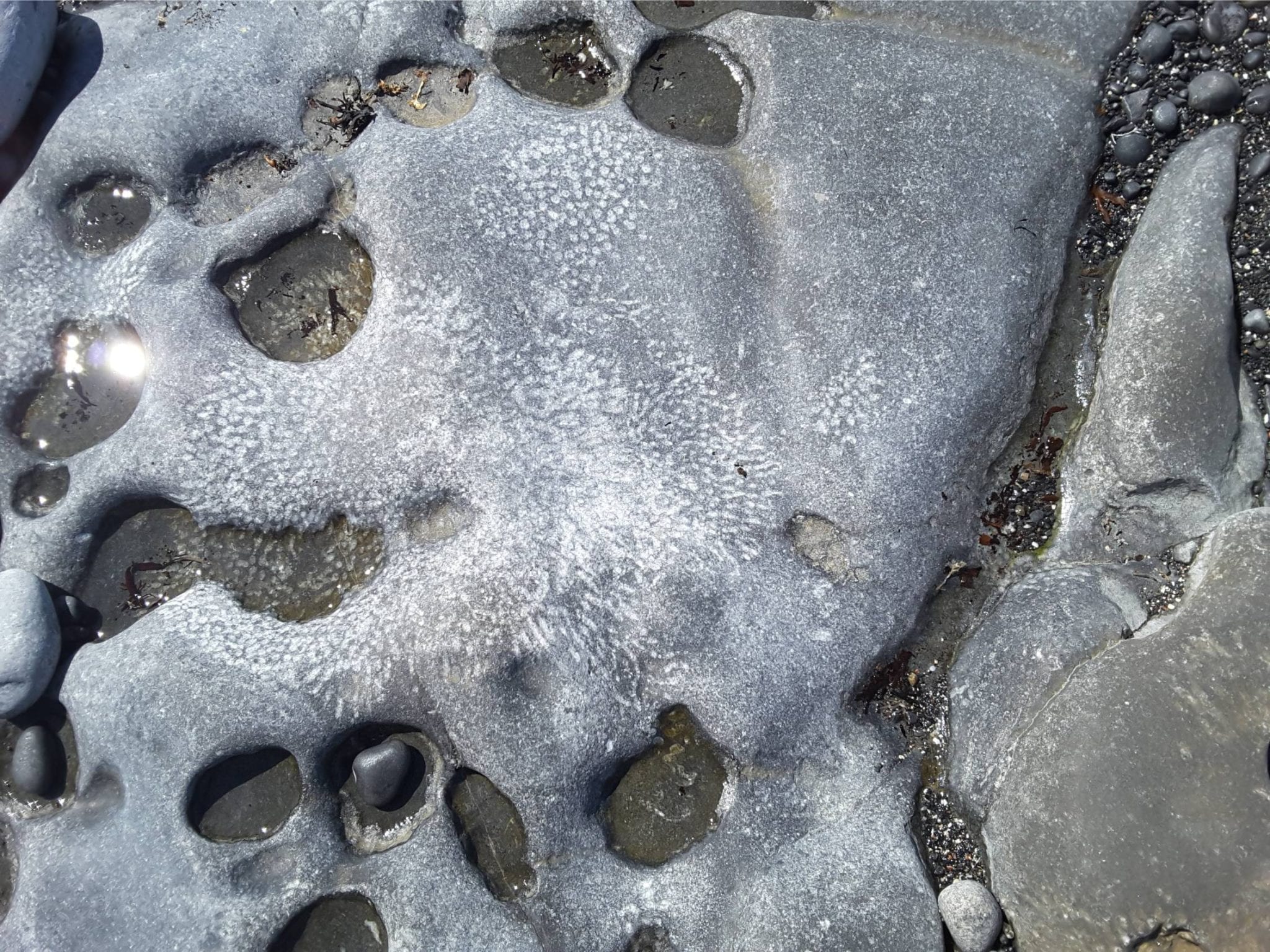
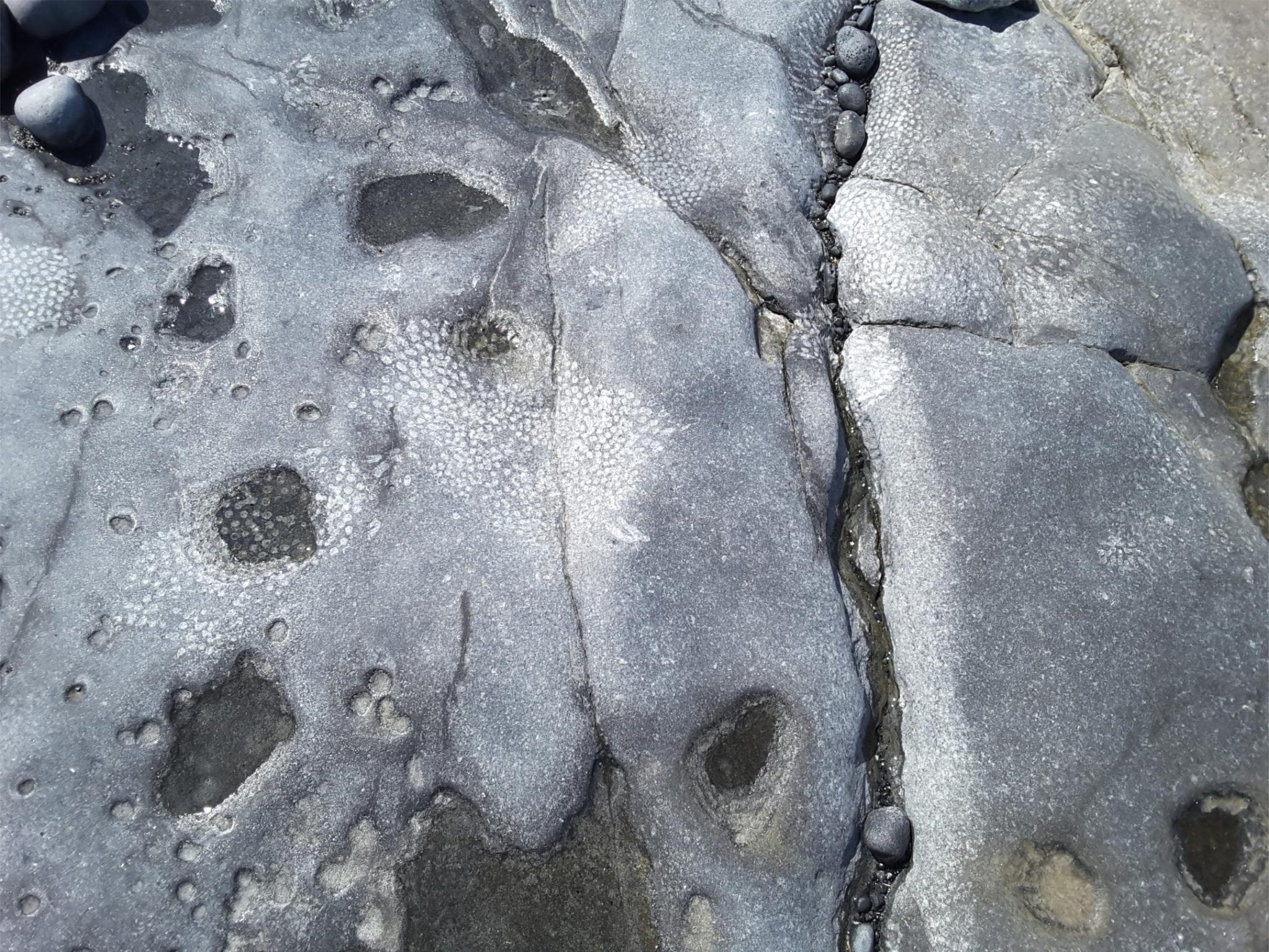
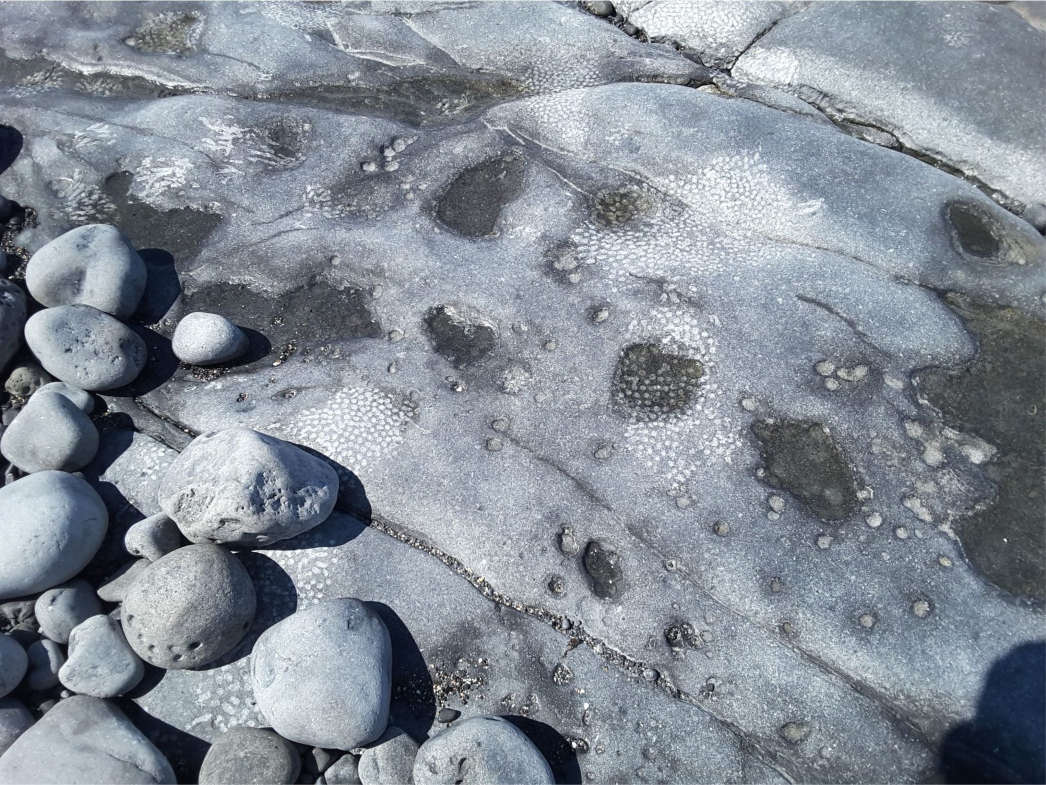
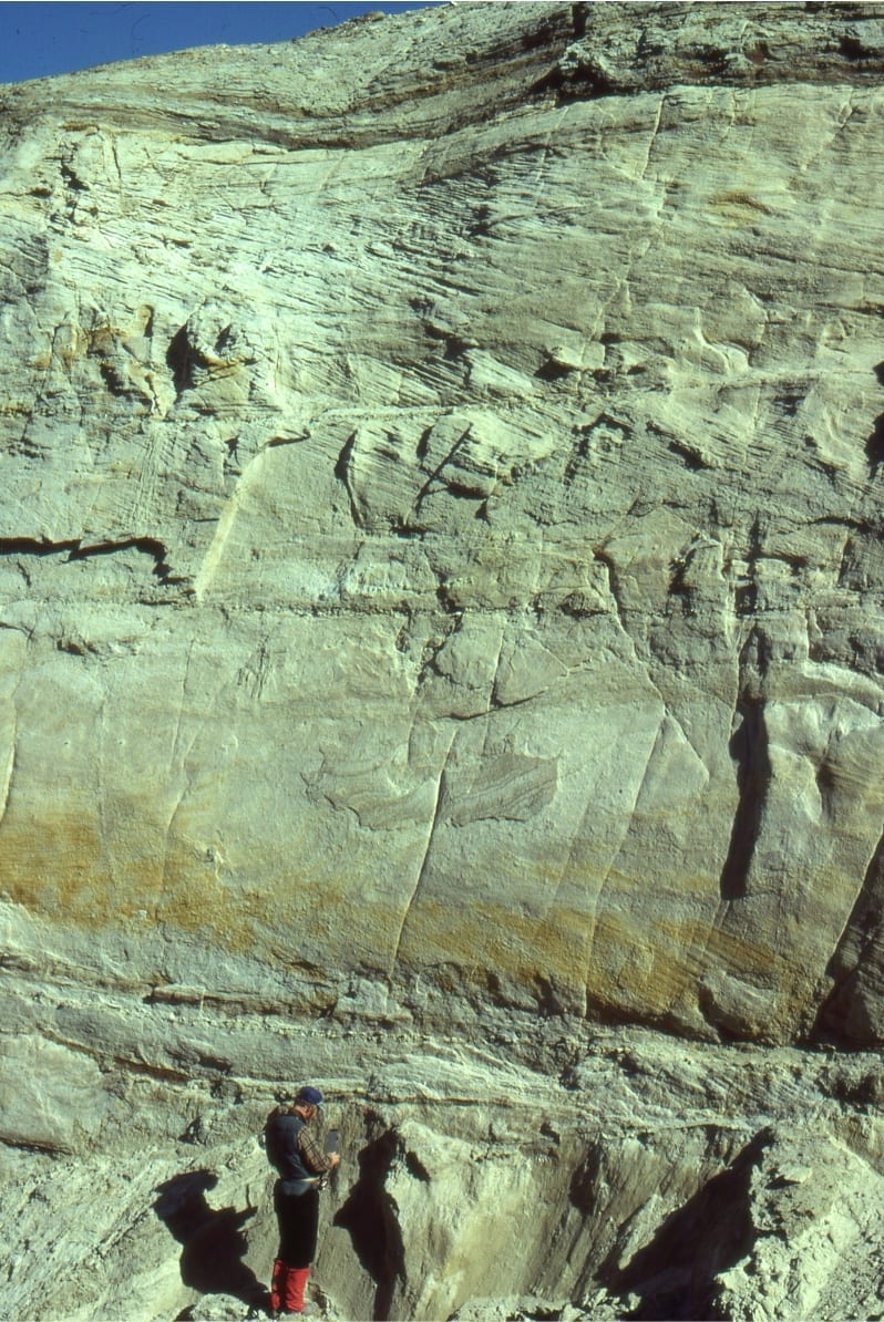
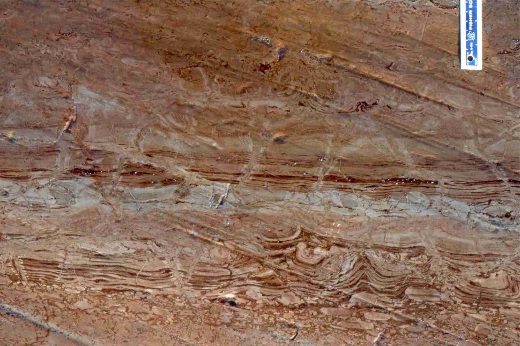
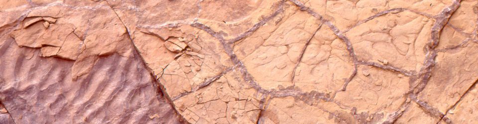
One of the more obvious examples of dilation is pressure solution, where certain minerals dissolve under compression, thus reducing rock volume. Cleavage forms in response to a combination of rock shortening and growth of metamorphic minerals like mica and chlorite. Stylolites, a relatively common structure in (non-metamorphosed) carbonates also represent pressure solution of calcite or dolomite, that thins rocks perpendicular to the principle compressive stress. A necessary condition for stylolitization is that the dissolved minerals must be removed from the area of compression; this involves mass transfer of the aqueous solutions. The boundaries of pressure solution are typically irregular, saw-toothed surfaces marked by dark insoluble minerals such as clay, quartz and feldspar.

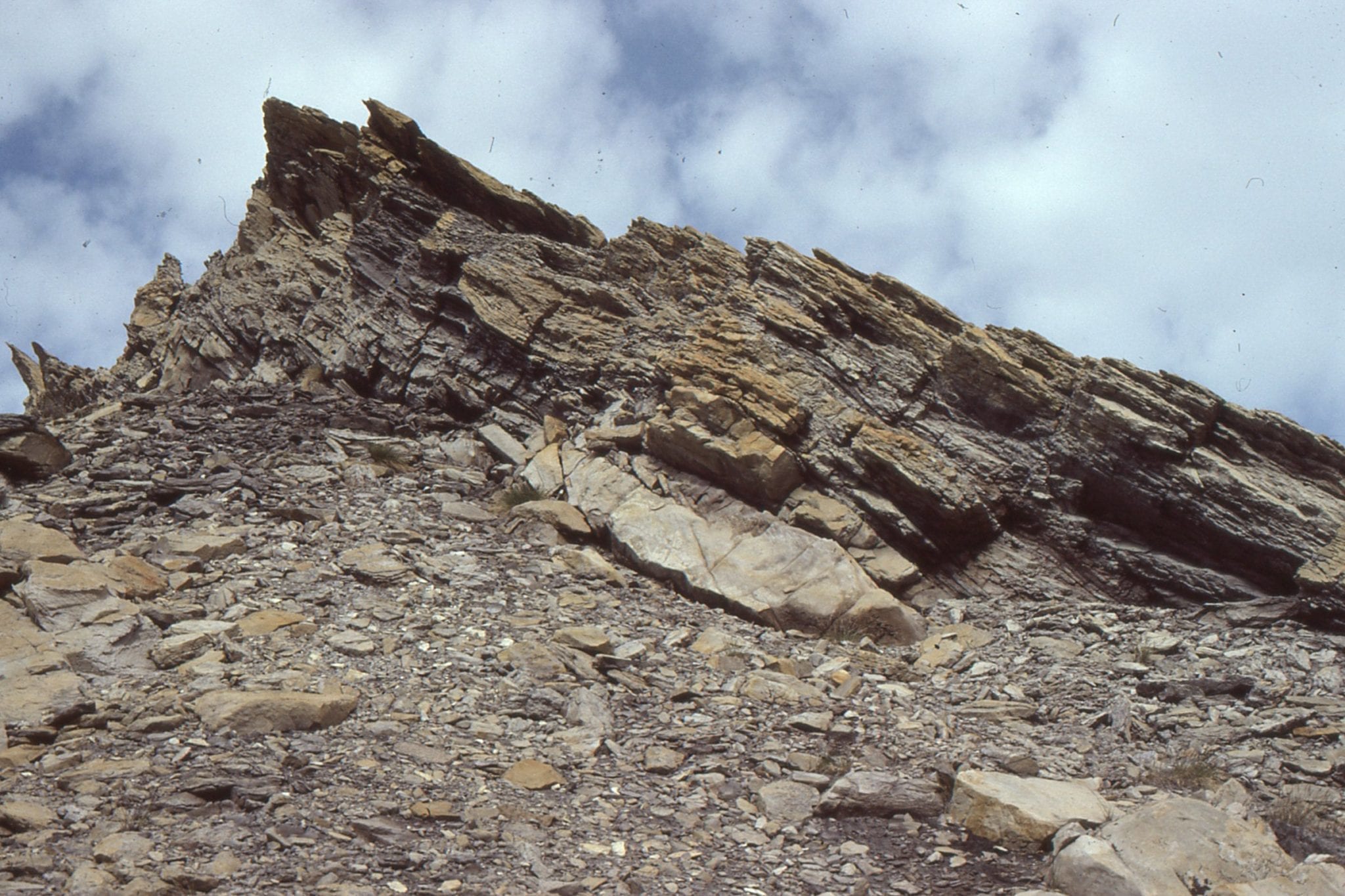
Kinematic indicators do not occur in isolation. For example, the Alberta Front Ranges (part of the Rocky Mountains) consists of a humongous stack of thrust sheets; all the structures associated with the thrusts such as hanging-wall and foot-wall folds, normal faults and ramps are kinematically linked. The indicators may change from one locality to another – from dislocation here to distortion there, but to make sense of this structural domain, there needs to be consistency among all the indicators, whether you are looking at a thin section, an outcrop, or entire mountain belt.

Using S and Z folds to decipher large-scale structures

Leave a Reply

This post is part of the How to… series

A problem frequently encountered when mapping structurally deformed rocks is deciding whether the fold you see in outcrop is part of a larger structure – an anticline or syncline, overturned or recumbent, plunging? The problem is exacerbated if stratigraphic facing (younging) criteria are absent or ambiguous. Fortunately, there is a solution to the problem based on fold asymmetry.

Large folds commonly have smaller-scale folds in their limbs and crest. They are usually referred to as higher-order (2nd, 3rd order etc.) or parasitic folds. They form during flexure of layered rock where slip occurs between rock layers – a mechanism called flexural slip. Structural geology teachers frequently use a soft-cover book to demonstrate this mechanism; bend the book into a fold and watch the slip between adjacent pages that is required to accommodate extension on the outer arc of the fold and shortening on the inner arc.

Parasitic folds are common in deformed sedimentary rocks where slip takes place along bedding planes or between layers with contrasting strength, such as mudstone and indurated sandstone (mudrocks have abundant clays and micas that are prone to slip and shear). The example below shows an anticline (1st-order structure) and smaller 2nd-order folds developed in a relatively weak layer. The 2nd-order folds have asymmetries related to the sense of slip on each fold limb and are called S- and Z-folds. Note that the 2nd-order M-folds in the hinge are symmetrical and in this example, upright.

The difference between S- and Z-folds lies in their sense of rotation, or vergence. The long limbs of S-folds are connected by a shorter limb that implies counter-clockwise rotation or sense of displacement; the opposite applies to Z-folds. Thus, the vergence of parasitic folds is towards the hinge line (or zone)

S- and Z-folds are three dimensional structures and will have hinge lines (or fold axes if we consider them to be cylindrical folds) and axial surfaces that can be measured. Another important property of parasitic folds is that their hinge lines (or fold axes) are parallel (or approximately so) to the hinge line of the 1st-order fold.

A note of caution; the sense of fold rotation-displacement will change if a fold is viewed from the opposite direction (i.e. S-folds will appear as Z-folds). Hence it is necessary to indicate the direction in which observations are made. Where possible, folds should be viewed down-plunge.

The geometric disposition of S- and Z-folds is extremely useful for deciphering large-scale folds, particularly when exposure is incomplete (as is commonly the case). The diagram below shows a scenario, where small folds are exposed in two outcrops.

Our view indicates the left outcrop is a Z-fold; the one on the right an S-fold. We can also determine the general attitude of the 1^st-order fold limbs from dips and strikes on associated beds. If 1^st-order fold-closure is beneath the surface, then it is a syncline (or synform if we don’t know facing direction); if above, an anticline or antiform. Both parasitic folds indicate vergence above the outcrops. If the structure was a syncline then the vergence should be in the opposite direction. The structure is therefore an antiform. If we have good facing direction data we could confirm the 1^st-order structure is an overturned anticline (stratigraphy in the right outcrop is overturned).

Some other posts in this series:

Measuring dip and strike

Stereographic projection – the basics

Stereographic projection – unfolding folds

Stereographic projection – poles to planes

Faults – some common terminology

Atlas of modern coral reefs

Leave a Reply

This is a companion post to the Atlas of Cool-water carbonates

Modern coral reefs and carbonate platforms provide the key ingredients of process and product to interpret ancient carbonate deposits. Here we can observe directly the relationship among all those processes – biological, physical, chemical – that contribute to the construction of solid rock.

Contributors

The inaugural collection of images for modern coral reefs has been generously donated by Charlie Kerans, the Department Chair and Robert K. Goldhammer Chair in Carbonate Geology in the Department of Geological Sciences, Jackson School of Geosciences, The Univeristy of Texas at Austin. Charlie is a carbonate specialist. I first met Charlie at Carleton Univeristy in Ottawa, where we shared an office whilst both of us were undertaking Doctoral research. Both of us worked on Precambrian rocks; Charlie on carbonates. He hasn’t stopped looking at carbonates.

The collections here are from Palancar Caves, and Columbia reef, Cozumel, off the Caribbean coast of Yucatan Peninsula. They are popular diving spots, for good reason as the images will attest. The water is clear and there is great diversity of reef and off-reef fauna and flora. It is a fantastic location to look at analogues for ancient reef systems – hard corals, soft fan corals, algae (particularly Halimeda), sponges, bryozoa, fish.

I’d be grateful for any corrections and clarifications to the species identifications.

The Atlas, as are all blogs, is a publication. If you use the images, please acknowledge their source (it is the polite and professional thing to do). Copyright of images is retained by the owner, as indicated. Contact Charlie for further information (link above).

This link will take you to an explanation of the Atlas series, the ownership, use and acknowledgment of images. There, you will also find links to the other Atlas categories.

Click on an image for an expanded view, then the ‘back page’ arrow to return to the Atlas.

The images: Palancar Cave, Cozumel

Columbia Reef, Cozumel

This reef, part of the reef system along the west coast of Cozumel, is located a little south of the Palancar reefs.

Identifying paleocurrent indicators

3 Replies

Sedimentary structures that indicate paleoflow. Measuring and plotting paleocurrent indicators are treated in a separate post.

This post is part of the How To… series

Sediment that is moved along a substrate (e.g. the sea floor, river bed, submarine channel, wind-blown surface) will commonly generate structures that record its passing. Sedimentary structures that preserve directionality (paleoflow) are indispensable for deciphering whence the sediment came and where it went; for interpreting sedimentary facies (local scale) and sedimentary basins (regional scale). Paleocurrents are a measure of these ancient flows.

A single structure, such as a ripple will give a unique measure of paleoflow at a certain point in space and time. An important question for this single piece of data is – how relevant is it to the bigger picture of sediment dispersal? To get a sense of regional flow and sediment transport patterns, we need many measurements so that we can tease the overall pattern of flow from whatever local variations might exist.

We can illustrate this central problem by looking at flow in a fluvial meander belt with depositional settings like the main channel (arrows), point-bars and adjacent flood plain. This snapshot in time shows clearly the huge variation in local flow directions. We also need to account for other ‘snapshots’ in time, because even at a local scale (e.g. one meander bend and point-bar), the directions of flow and sediment transport will vary from flood to low water stage. We can try to circumvent this problem if we measure a large number of flow directions over an equally large area of the river and floodplain. In modern drainage basins this is straight forward but for the rock record, exposure is likely to be discontinuous and even structurally disjointed.

Structures indicating unique flow directions

Subaqueous dunes and ripples: These bedforms are built by 2-dimensional (straight-crested) dunes and ripples. Hence, the boundaries between adjacent crossbed sets tend to be planar (cf. trough crossbeds). Flow direction is approximately at right angles to dune or ripple crests.

Trough crossbed, or 3D subaqueous dunes Spoon-shaped troughs filled by migrating, sinuous dunes produce trough crossbedding. This kind of crossbed is common in confined, channelized flow (e.g. fluvial and tidal channels). The mean flow direction is along the axis of the trough.

Left: Festooned trough crossbeds exposed approximately parallel to bedding. Paleoflow is the direction of the hammer handle Proterozoic Loaf Fm.). Right: Cross-section view of multiple trough crossbeds – only apparent flow directions can be surmised from outcrop (Eocene Buchanan Lake Fm.).

A caution about wave-formed ripples; This bedform does not arise from bedload transport in flowing currents, but from wave orbitals. Wave ripples are not paleocurrent indicators. However, wave ripple crests will be oriented approximately parallel to the strike of the ancient shoreline.

Imbrication Flat and platy clasts are commonly oriented by strong currents, such that the ‘plates’ dip upstream. These fabrics are common in gravelly fluvial deposits.

Imbricated platy cobbles and pebbles in a modern stream. Flow is to the right.

Flute casts Flutes originate from erosion of a soft, commonly muddy substrate and are filled with sand – they are part of the overlying bed and are usually seen as casts on the sole of the overlying bed. Flow direction is towards the open, shallow end of the flute.

Large flute casts on a turbidite bed sole (Omarolluk Fm, Belcher Islands). Flow was from top left to bottom right

Structures indicating ambiguous flow directions:

Groove casts Objects dragged across a soft substrate by strong currents (e.g. bottom currents, turbidity currents) will scour linear grooves that become filled by the overlying sedimentary layer. Like flutes, they are usually seen as casts on the soles of beds. In the absence of other indicators, the two possible paleoflow directions are 180^o apart.

Groove casts on a bed sole, indicate flow in either direction. other criteria, like flute casts, are need to specify unambiguous flow directions.

Parting lineation These are subtle structures 2 or 3 grains thick, that are visible only on exposed laminated bedding. The word ‘Parting’ refers to rock breakage along planar laminations. Parting lineation is attributed to high flow velocities where the long axes of sand grains become aligned (in Flow Regime terminology this corresponds to Upper Plane Bed conditions). Paleocurrents are measured parallel to the long direction of parting, but like groove casts, are ambiguous.

Paleoflow indicated in this parting lineation was either to the left or right.

Current alignment of elongate fossils, rod-shaped clasts, or bits of wood can generally be treated like groove casts in terms of their paleocurrent value. There are exceptions; for example turreted gastropods may be aligned with their apices pointing downstream. The example shown here shows fairly consistent alignment of Permian Fusulinid foraminifera parallel to the prevailing flow (but the actual flow direction is ambiguous).

The classic text that deals with paleocurrent analysis is – Potter, P.E. and Pettijohn, F.J. (1977) Paleocurrents and Basin Analysis. 2nd Edition, Springer-Verlag, New York, 425 p.

Some more useful posts in this series:

Measuring a stratigraphic section

Measuring and representing paleocurrents

Crossbedding – some common terminology

The hydraulics of sedimentation: Flow Regime

Determining stratigraphic tops

Leave a Reply

a.k.a. Stratigraphic way up, or younging direction

This post is part of the How To… series

Stratigraphy is all about succession in the rock record – which events preceded other events; which is older, which younger. Nicolas Steno (1638-1686) surmised, and four centuries of geologists since have confirmed that in an uninterrupted succession of strata, the youngest layer is at the top. However, tectonic hiccups and upheavals have frequently turned successions of strata sideways or on their head. In this case, knowing which way is ‘up’ will confirm which strata were overturned. Continue reading →

Stereographic projection – unfolding folds

Leave a Reply

Restoring paleocurrent trends to their pre-deformation orientations

This post is part of the How To… series

Sedimentary strata are commonly deformed. If we assume that the original depositional dip was close to horizontal (this is a reasonable assumption, although there are exceptions) then we need to account for structural dip. This is important if our sedimentary analysis includes measurement of paleocurrents, depositional dip and strike (e.g. ancient shorelines, rivers), or any paleogeographic determination.

Two methods are outlined here: the standard stereographic projection method that is usually done back in the lab unless you are lucky enough to have access to the internet in the field; and a quick field method using a field note book, pencil and compass; this method can only be used in strata folded by a single phase of deformation.

Stereographic method

In the simplest case (diagrams below), strata containing flute casts have been folded into a syncline with a horizontal fold axis; we need to correct the for dip in the fold limb to find the original orientation of the flute cast. Bedding strikes 080^o (N80E), dip 40^oN; the flute cast plunges 38^o at 315^o (N45W).

On a transparent overlay, plot the plane (strike and dip) and the line (orientation and plunge) representing the flute cast (it will be a point on the great circle) on the stereonet. To return the plane to its original pre-fold orientation, it must be rotated about its strike; the next step is to move the great circle back to its original plotting position. When the plane is rotated to horizontal all points on the great circle will move along small circles to the stereonet perimeter. The point representing the flute cast is now in its original orientation – here 332^o, or N28W. The difference between the uncorrected and corrected bearing is 14^o.

Direct field method

You can use this method when sedimentary structures (or any linear trend) are exposed on bedding planes. It basically performs the same task as a stereonet correction.

Place a hard, flat surface on bedding – hard-cover note book or board are good – with the long edge oriented along strike. Place a pencil or similar straight-edge on the surface such that it is aligned with the structure of interest (flute long axis, ripple trend etc). Rotate the book about its long edge (i.e. about the strike) until it is horizontal – make sure the straight-edge doesn’t move. Holding the book and straight-edge in place, measure the bearing.

If you are not convinced about the accuracy of the field method, check it against the stereonet correction. You will find with practice, and not a little care, that direct field measurement provides excellent results.

Some other posts in this series:

Measuring dip and strike

Solving the three-point problem

Stereographic projection – the basics

The Rule of Vs in geological mapping

Folded rock; some terminology

Solving the three-point problem

Leave a Reply

A graphical method for solving the three-point problem

This post is part of the How To… series

Determining the orientation of a plane given the points for three intersecting wells.

Mapping is the essence of geology. Geology maps provide the wherewithal to decipher the time and space organization of Earth’s solid and fluid spheres. We map the outer veneer by directly observing rocks and fluids, ‘walking out’ rock units, measuring, sampling and imaging as we go. More recent tools include all manner of remotely sensed data and satellite imagery (seismic, Lidar, radar, Landsat). We apply the same tools to map other planetary surfaces, although the walking-out is done by remotely controlled rovers.

Subsurface mapping is the essence of all explorations for aquifers, hydrocarbons, minerals, geothermal energy and geotechnical constructions. Subsurface mapping provides us with a deeper (sic) understanding of how the Earth works. Subsurface mapping is entirely dependent on remote sensing (e.g. seismic, gravity, radar) and borehole probing.

The orientation of geological planes in the subsurface is no less important than in surface mapping, but the database is commonly one-dimensional (e.g. borehole depths and lithologies). For example, a zone of mineralization at depth lies beneath an unconformity; knowing the orientation of the unconformity plane will give us more confidence predicting the trend of mineralization (assuming the unconformity is reasonably flat). To solve the problem, we need depths from three borehole intersections with the plane. The solution is commonly referred to as the 3-point problem. It is based on an understanding of dip and strike.

Geometric calculation of dip and strike in a 3-point problem

A graphical solution is shown in the animation. You need paper, a ruler and a protractor. This method requires the horizontal and vertical (depth or elevation) scales to be the same (no vertical exaggeration). Normally the construction would be done on the plane itself (i.e. 2-dimensional) – here the 3-dimensional view has been added to help you visualize the problem.

The animation was made from still images: use the pause and play buttons as you work through the exercise.

Some other useful posts in this series:

Measuring dip and strike

Stereographic projection – the basics

Stereographic projection – unfolding folds

The Rule of Vs in geological mapping

Folded rock; some terminology

Marie Tharp and the mid-Atlantic rift; a prelude to plate tectonics

Leave a Reply

The history of science is littered with the misplaced contributions by women, contributions that at best were pushed aside or ignored, and at worst thought of as shrill outbursts. Witness:

Rosalind Franklin’s fraught journey to DNA’s double helix,

the recent unveiling of Eunice Foote’s experimental discovery of the greenhouse effect of CO₂, and
Bell Bernell’s discovery of pulsars,

as corrections to a history where women found it difficult to escape the status of ‘footnote’. We can add Marie Tharp (1920-2006) to the growing list of corrections. In 1952 Tharp discovered the central rift system in the mid-Atlantic Ocean ridge (that later would become a critical component of sea floor spreading and plate tectonics) but for many years was regarded as a minor player in the burgeoning, post-war field of oceanography.

During the War, Tharp in her early twenties took advantage of opportunities to engage in university study, openings in science and engineering left by men who had gone to battle. She completed a Master’s degree in geology, but given that geology is a field-based discipline, and that women weren’t supposed to go into the field, she extended her studies to a Master’s in mathematics. In 1948 Lamont Geological Laboratory (now Lamont Doherty Earth Observatory) hired 28 year-old Tharp to draft maps of the Atlantic ocean floor, based on the growing database from SONAR and historical soundings. She worked with well-known geologist-oceanographer Bruce Heezen, who spent much of his time at sea. It must have been tedious work, but she counted herself lucky to have a position at all. This was a time when very few American universities (or anywhere else for that matter) offered science and engineering positions to women; a time of patriarchal condescension – “Mad Men” versus “Hidden Figures”.

Tharp poured over depth and positional data for years, constructing 2-dimensional profiles of the Atlantic Ocean floor. She was aware, as other oceanographers were that an elevated region of sea floor apparently separated east and west Atlantic. This was initially mapped in 1854 by US Navy oceanographer, geologist and cartographer Matthew Maury, and later confirmed with depth soundings taken during the HMS Challenger expeditions (1873-1876 – Challenger had 291 km of hemp onboard to do this kind of thing; the ridge is generally deeper than 2000m). Tharp wasn’t surprised to find the Atlantic ridge on her profiles. What did catch her attention was the rift-like valley in the central part of the ridge; a geomorphic structure that was consistent through all her profiles. She immediately recognized the importance of this, because it implied significant extension, a pulling apart of Earth’s crust in the middle of the ocean. At the time, the general consensus was that ocean floors were relatively benign, featureless expanses. Her discovery indicated otherwise.

According to Tharp’s bio the response by Heezen and his colleagues was that she was being a typical woman – you know, “girl talk”. One can imagine the coffee room banter; ‘she’s great at drafting cross-sections but should leave the interpretation to the more learned’.

However, after some months and more profiles all showing the same rift- like structure, Heezen gradually accepted that this was real. A turning point for Heezen was the coincidence of several mid-ocean earthquake epicenters along the ridge. This was mid 1953. He understood its potential significance, particularly for those who thought that the hypothesis of continental drift had some credence (Heezen was not initially one of those people).

Ocean bathymetry studies in other basins in the early 1950s (Indian Ocean, Red Sea) revealed similar mid-ocean rifts. Tharp had by this time surmised that a rift valley coursed its way almost continuously the entire length of North and South Atlantic, a distance of 16,000 km; it was the largest continuous structure on Earth. The Lamont Doherty group gradually realized that the Atlantic structure, together with those discovered in other ocean basins, represented a gigantic Earth-encircling system of mid-ocean rifts, more than 64,000 km long.

Heezen presented their research to a 1956 American Geophysical Union conference in Toronto. Marie Tharp barely received a mention. She did co-author a few subsequent publications as an ‘et al.’, but it was a kind of ‘also ran’; the accolades and approbation went Heezen’s way.

Tharp was fired by the Laboratory, the victim of a spat between Heezen and Lamont boss Maurice Ewing, but she continued to develop the maps at home. Marie continued to work in the background, as the humble and grateful recipient of a job she considered to be fascinating; “I worked in the background for most of my career as a scientist, but I have absolutely no resentments. I thought I was lucky to have a job that was so interesting”.

Marie Tharp was named one of the four great 20^th century cartographers by the Library of Congress in 1997, was presented with the Woods Hole Oceanographic Institution Women Pioneer in oceanography Award in 1999, and the Lamont-Doherty Heritage Award in 2001.

There is no question that Tharp’s discovery influenced the promotion of Continental Drift in the geoscience community. Alfred Wegener’s bold hypothesis (1915) had one major problem – there was no known mechanism that could move oceanic crust and continents around, like some precursor shuffle to a jigsaw puzzle. In 1929 Arthur Holmes posited a mechanism that involved large convection cells in the mantle, but this too lacked an important degree of empirical verification. Discovery of the mid-Atlantic rift provided a solution to this vexing problem, and in 1962 Harry Hess proposed that new magma, via mantle convection cells, was erupted from mid-ocean rifts allowing oceanic crust to spread outwards. This was Sea Floor Spreading, a precursor to the grand theory of Plate Tectonics – the tectonic shift in geological thinking wherein oceanic crust is created at mid-ocean rifts and consumed down subduction zones, with the continents playing tag.

Marie Tharp’s doggedness in her belief and understanding of mid-ocean rifting is now celebrated. It’s taken a few decades, but she is no longer a footnote.

Atlas of the Burrens, County Clare

Leave a Reply

The Burrens – a limestone karst landscape

Here’s a selection of photos from the Burrens of County Clare, Ireland. Carboniferous limestones, in a glacio-karst landscape: karst structures, landscapes, vegetation, and fossils, from inland and shoreline exposures.

There is an article on the Burrens here.

The Atlas, as are all blogs, is a publication. If you use the images, please acknowledge their source (it is the polite, and professional thing to do).

This link will take you to an explanation of the Atlas series, the ownership, use and acknowledgment of images. There, you will also find links to the other Atlas categories.

Click on the image for an expanded view, then ‘back page’ arrow to return to the Atlas.

New Quay and Abott Hill:

Burrens landscape north of Boston (a few km south of New Quay. Limited soil cover on the limestone bedrock, and scrubby vegetation. Typical rounded hills of limestone in the background.

Views north of the estuary and Galway Bay from Abott Hill (between New Quay and Kinvara)

Clints and grykes, Abott Hill, typical Burren karst structures. Right image: smaller scale dissolution rills.

Typical Burren hill and more fertile lowland valley near New Quay

Flaggy Shore (near New Quay):

Salt corrosion and erosion of limestone along Flaggy Shore, has modified the clints and grykes. Some erosion is caused by potholed cobbles.

Clints and grykes on the raised shore platform along Flaggy Shore

Abundant colonial Visean corals, best seen on semi-polished surfaces along the Shore. These views are oblique and cross-sections of coral columns.

Black Head:

The raised shore platform at Black Head (below the road) consists of several benches elevated during post-glacial rebound.

Clints and grykes, typical karst structures, are well developed all over the Black Head platform, controlled by dominant fracture trends. They provide succor and shelter to a variety of small shrubs and wild flowers.

Smaller scale dissolution limestone rills are common along exposed gryke walls

Polished limestone along the Black Head shore reveal fossil corals and brachiopods. The stepped landforms are controlled by dominant fracture trends.

Tidal pools, regularly flushed by incoming tides.

Bouldery storm ridges have been pushed over the Black Head platform by Atlantic storms.

Typical vegetation eking out a living in the grykes. Succulents (left) are most common close to the shore.

Atlas of beach, lagoon, bar, estuary, tidal flats

Leave a Reply

Shallow marine – estuarine – tidal flat – lagoon and coastal dunes

This collection of images spans the shallowest marine environments including beach, lagoon-bay with all the associated environments such as sand-spits and barrier-bars, tidal flats, estuaries and coastal dunes. Where possible I have paired modern analogues with ancient examples.

The Atlas, as are all blogs, is a publication. If you use the images, please acknowledge their source (it is the polite, and professional thing to do).

This link will take you to an explanation of the Atlas series, the ownership, use and acknowledgment of images.

Click on the image for an expanded view, then ‘back one page‘ arrow to return to the list

The images:

Tairua estuary, east coast Coromandel Peninsula, New Zealand. Two images taken during falling tide, exposing attached and semi-detached sand-shell bars. The main channel is at bottom of each image.

Raglan ebb tidal delta, bedforms on the platform attached to the permanent shoreface

The estuary on the south side of Galway Bay, County Clare, Ireland, near New Quay. The boulder-cobble beach consists almost entirely of Burrens limestone (Carboniferous). Left view from Abbot Hill.

Mudflats and algae, Kinvara, at the head of the estuary, south side Galway Bay.

Karst in Burren Limestone at Flaggy Shore, New Quay, County Clare, has been accentuated by salt corrosion and mechanical erosion. It is overlain by boulders of locally derived Carboniferous limestone

Boulder storm ridge at Black Head, County Clare – the heart of the Burrens. All boulders are locally derived Carboniferous limestone

Potholes in Burren Limestone, Flaggy Shore, County Clare.

Sea grass, ripples, and burrow excavations in a tidal pool, Flaggy Shore, County Clare

Large, 2D dunes, intertidal Minas Basin, Fundy Bay

Shallow subtidal to intertidal, 2D subaqueous dunes, Rowatt Fm, Belcher Islands (Aphebian, about 2 billion years old). Hammer for scale.

Cross-sectional view of 2D subaqueous, intertidal dunes, showing complex migrating dune-formed crossbedding, and dune reactivation, Rowatt Fm, Belcher Islands (Aphebian, about 2 billion years old). The sands are mixed siliciclastic-carbonate (dolomite).

Reactivated 2D dunes with superposed ebb tide ripples, Minas Basin, Fundy Bay

Proterozoic tidal inlet, showing cross-section of reactivated subaqueous dunes (mid image), possible herringbone crossbeds, and smaller ripples. Rowatt Fm, Belcher Islands (about 2 billion years old). Lens cap bottom right.

Multiple dune sets, intertidal, Minas Basin, Fundy Bay

Sandy tidal flat ripples, Minas Basin, Fundy Bay

Paleocene, straight crested and bifurcating intertidal ripples, Expedition Fm, Axel Heiberg Is;and, Canadian Arctic

Straight-crested ripple train in Paleocene intertidal deposits, Expedition Fm, Axel Heiberg Island, Canadian Arctic. Hammer left-mid image.

Flood tide ripples over-ridden by smaller ebb tide ripples sets. Minas Basin, Fundy Bay

Interference ripples in Proterozoic tidal flat facies, Belcher Islands

Large 2D and 3D dunes, and superposed run-off ripple sets, Minas Basin Fundy Bay

Tidal flat, interference ripples, Minas Basin Fundy Bay

Ebb tide run-off & reactivation of 3D dunes, Minas Basin Fundy Bay

Large 3D dunes, Minas Basin Fundy Bay

2D flood tide dunes and small ebb tide ripples, Minas Basin Fundy Bay

2D and 3D intertidal dunes, Minas Basin Fundy Bay

Eroded salt marsh cycles, Minas Basin Fundy Bay

Small meandering tidal channel in very muddy estuarine tidal flats, Whitford Estuary, south Auckland. Bank failure is common.

Salt marsh, sedges and small mangroves being transgressed and eroded by tidal flat. This is a modern example of a ravinement surface. Whitford, south Auckland

Eroded salt marsh deposits, transgressed by sandy tidal flat – beach. The erosion surface is a modern, active ravinement surface. Galveston, Texas.

Two examples of Paleocene tidal bedding (mostly lenticular and wavy bedding) interfingering with lagoon and marsh. Eureka Sound Group, Ellesmere Island

Paleocene tidal bedding interfingering with marsh-lagoon-bay sediment. On the right, the thicker sandstones may represent storm washovers into the bay. Eureka Sound Group, Ellesmere Island

Coarsening- and sandier-upward bay or lagoon subtidal to beach, cut by small tidal channels (lenticular sandstones). Eocene, Eureka Sound Group, Ellesmere Island.

Ebb tidal delta at the mouth of Waikato River, south Auckland.

Paleocene subaqueous dunes up to 2m amplitude, in tidal inlet-delta, overlain by thin tidal flat-salt marsh deposits. Expedition Fm, Axel Heiberg Island, Canadian Arctic

Large within-channel dunes in a tidal inlet associated with a sand spit facies; the spits and bars were attached to (paleotopographic) headlands across an unconformity eroded into Ordovician carbonates. Paleocene, Eureka Sound Group, Ellesmere Island.

Two views of the unconformity between Ordovician carbonates and Paleocene estuarine-tidal channel-spit facies. Eureka Sound Group, Ellesmere Island.

Typical beach stratification in an eroded berm; primarily laminated sets with low-angle truncations, parallel, or slightly inclined to the beach face.

Tidal inlet standing waves (antidunes) in an outgoing tide, Mangawhai Heads, north Auckland. The antidunes migrate up-current (against the current) and gradually build until they break, subsequently reforming.

Proterozoic tidal channel – inlet trough crossbeds; this outcrop gives a 3-dimensional view of individual sets. Paleoflow was into the image. Rowatt Fm. Belcher Islands.

Flaser, lenticular and wavy bedding in late Pleistocene deposits near Ihumatao, Auckland. White muddy sediment overlies and envelopes grey sandy ripples, and fills troughs between ripples.

Coastal dunes, Galveston coast, Texas

Washover fan breaching coastal dunes, Galveston coast, Texas

Paleocene washover fan sandstone associated with barrier island and tidal inlets (see images above from the same formation), Expedition Fm, Axel Heiberg Island, Canadian Arctic.

Stacked storm deposits associated with an upper tidal flat, each layer consisting of ripped up muds. Rowatt Fm, Belcher Islands. Proterozoic.

Mudcracks in salt marsh, Kaiua, NZ

Proterozoic supratidal desiccation cracks and voids in multiple layers of delicately laminated dololutite. Some curled slabs may be coated with crpytalgal laminae. A layer of storm-derived lutite rip-ups at the bottom of the image. Rowatt Fm. Belcher Islands. See below for a modern analogue.

Desiccated, curled, algal mats from a salt marsh near Galveston Texas. The mats are easily disturbed during high or storm tides.

Mangroves: Left image: stabilizing shell banks (storm ridges) adjacent a tidal Inlet, Auckland Harbour; Right image: in a salt marsh, Kaiua, bordering Hauraki Gulf.

Everglades Mangroves, Florida. A tangle of roots and pneumatophores that are living quarters for so many species. On the right, an epifauna of barnacles, small snails and bryozoa.

Everglades alligators, including the little guy on its parent’s head.

Gravel bar formed at the intersection between a high energy, West coast New Zealand beach, and the Tangahoe River mouth

Ripples on a sand flat, with concentration of heavy minerals from local rhyolites and dacites. Little Bay, Coromandel.

Geological Digressions

Earth science resources, images, glossaries, and SCICOMM for students and non-specialists

Tag Archives: scicomm

Kinematic analysis of deformed rock

Other useful links in this series…

Like this:

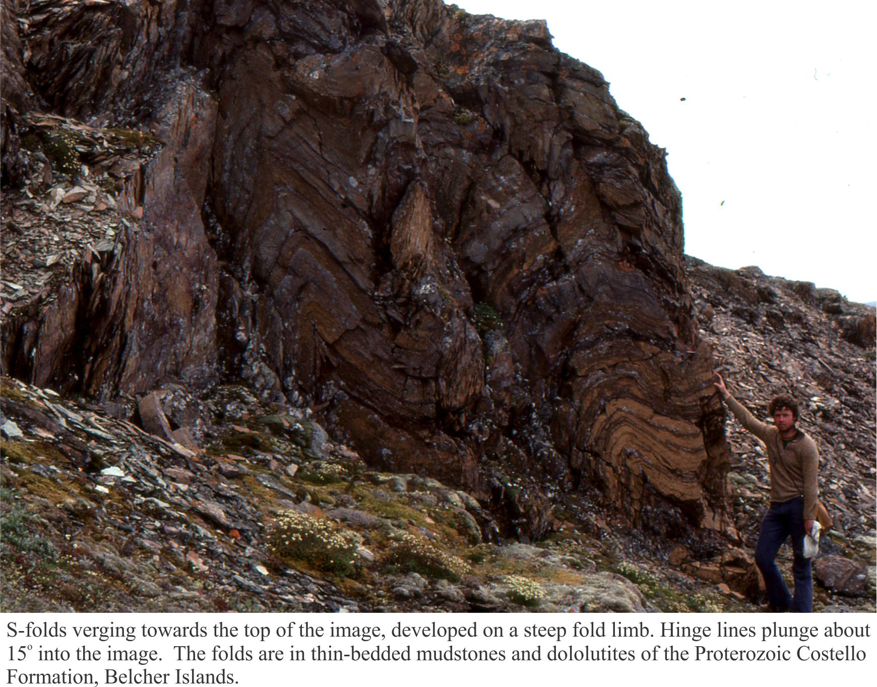
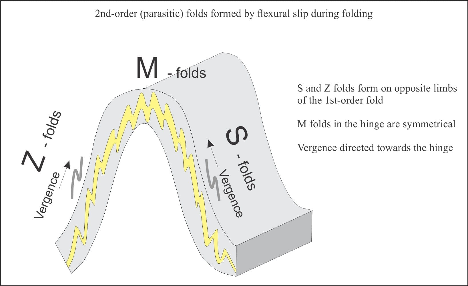
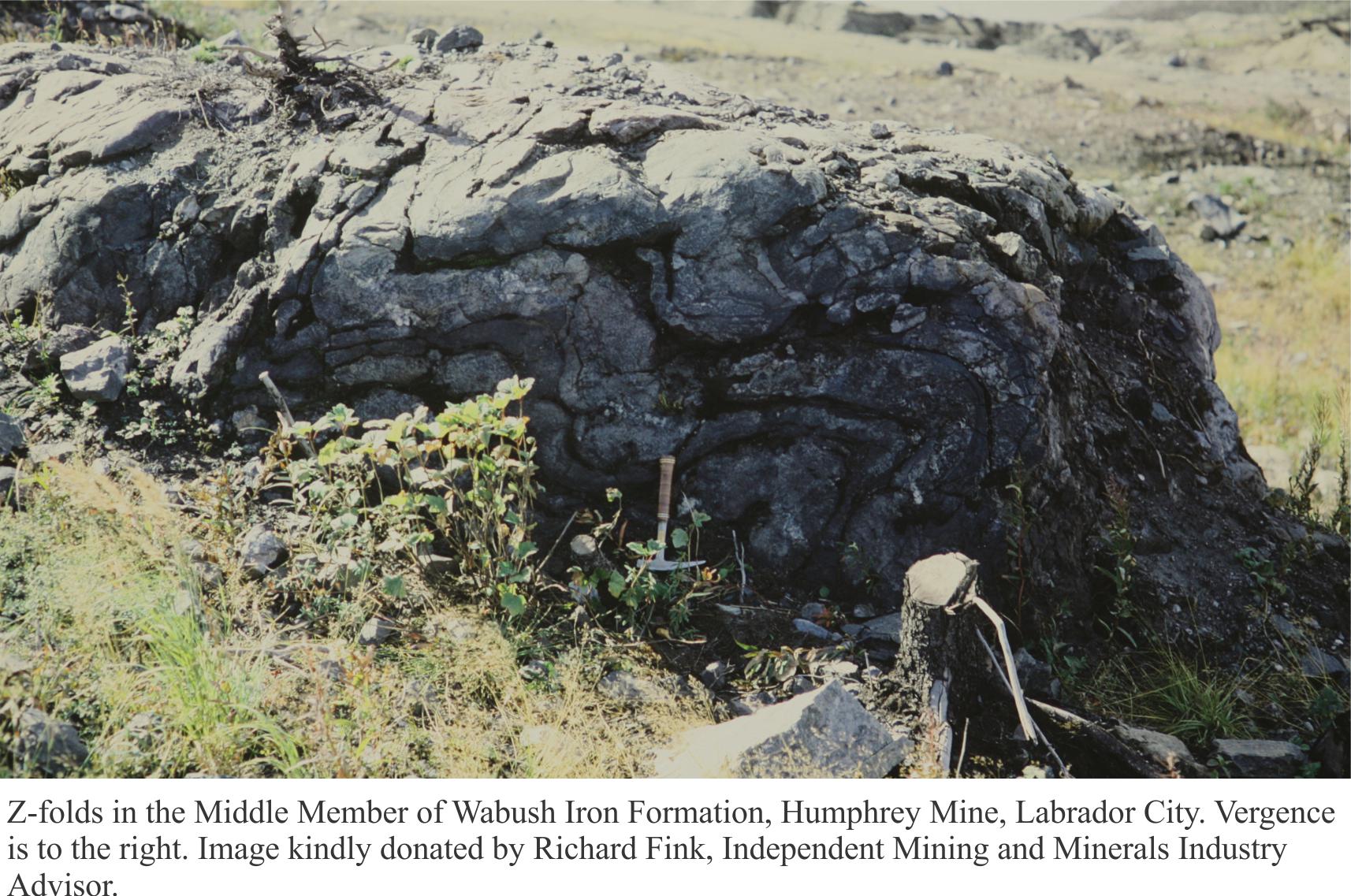
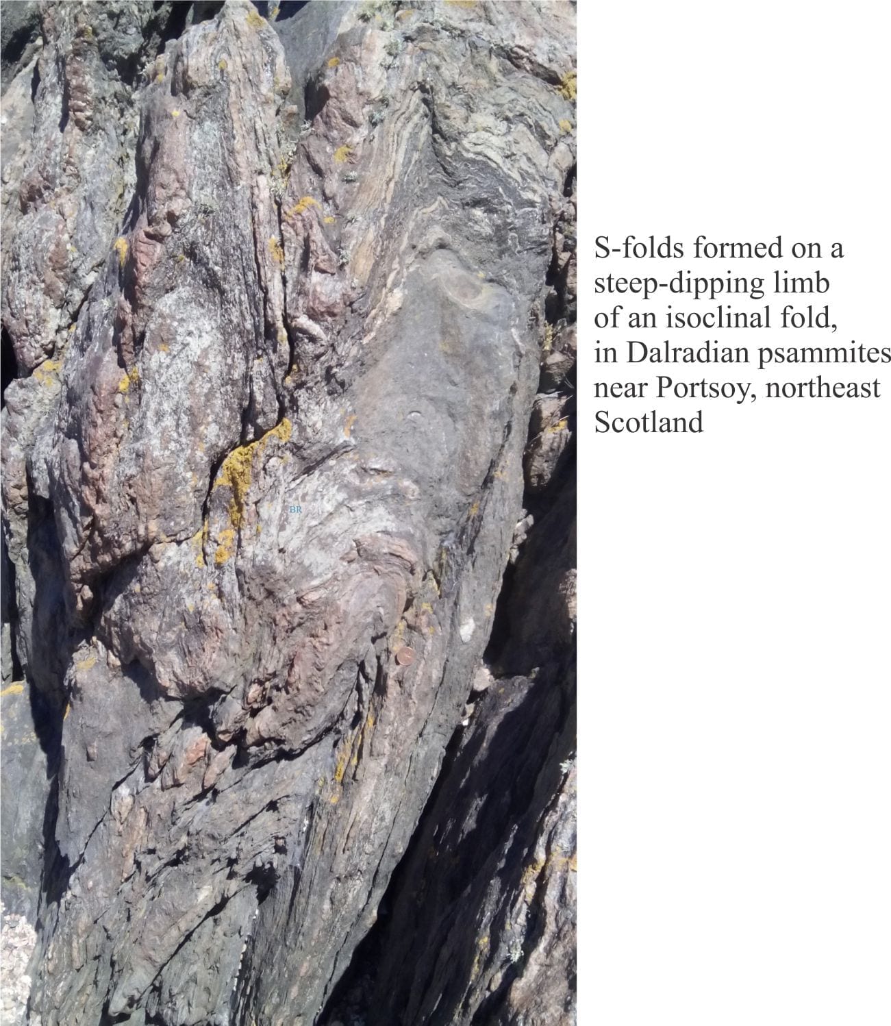
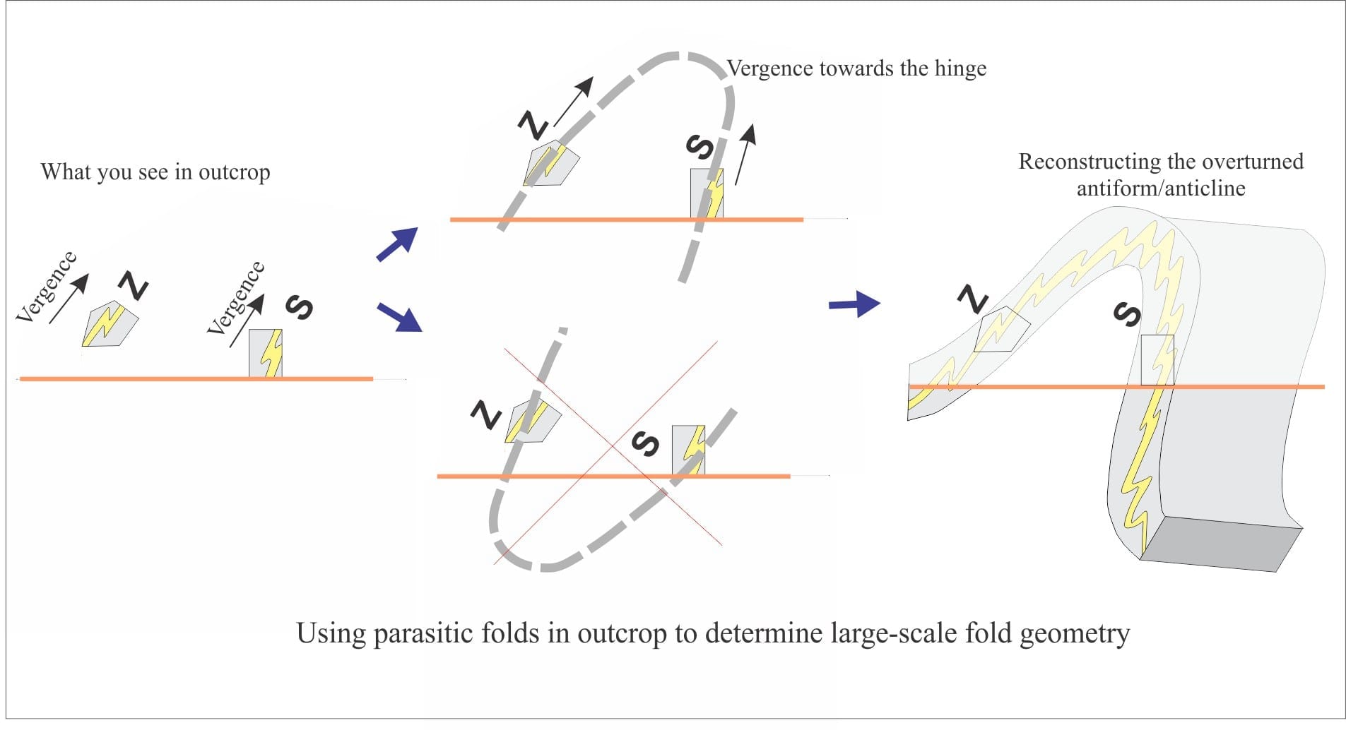
Using S and Z folds to decipher large-scale structures

Like this:

Atlas of modern coral reefs

Contributors

The images: Palancar Cave, Cozumel

Columbia Reef, Cozumel

Like this:

Identifying paleocurrent indicators

Structures indicating unique flow directions

Like this:

Determining stratigraphic tops

a.k.a. Stratigraphic way up, or younging direction

Like this:

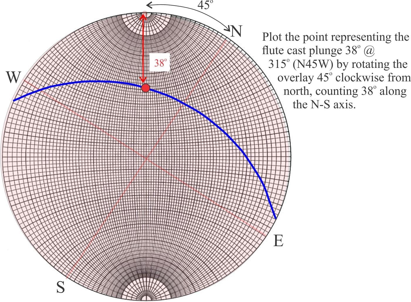
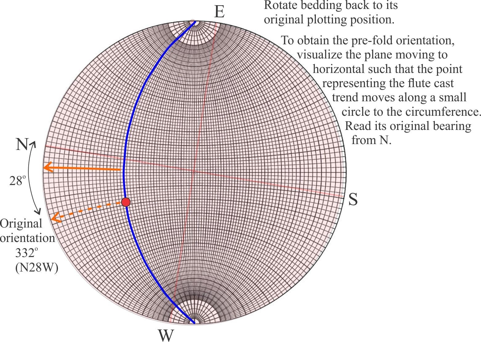
Stereographic projection – unfolding folds

Restoring paleocurrent trends to their pre-deformation orientations

Like this:

Solving the three-point problem

Like this:

Marie Tharp and the mid-Atlantic rift; a prelude to plate tectonics

Like this:

Atlas of the Burrens, County Clare

Like this:

Atlas of beach, lagoon, bar, estuary, tidal flats

The images:

Like this:

Other useful links in this series…

Share this:

Like this:

Share this:

Like this:

Contributors

The images: Palancar Cave, Cozumel

Columbia Reef, Cozumel

Share this:

Like this:

Structures indicating unique flow directions

Share this:

Like this:

a.k.a. Stratigraphic way up, or younging direction

Share this:

Like this:

Restoring paleocurrent trends to their pre-deformation orientations

Share this:

Like this:

Share this:

Like this:

Share this:

Like this:

Share this:

Like this:

The images:

Share this:

Like this: