 Space may well be the final frontier (there are one or two on earth that still require some work), but the space around our own planet is decidedly crowded. Folk at NASA’s Goddard Space Center (Maryland) estimate about 2300 satellites now orbit Earth; vehicles in various states of repair, use or disuse, of which a little more than 1400 are operational
Which leaves a lot of junk – euphemistically called ‘completed missions’. This level of traffic is certainly manageable, but for the added problem of more than 500,000 bits of real junk, flotsam and jetsam such as bits of satellites, spent boosters, dropped spanners, nuts and bolts, and satellites that disintegrate during missile target practice; this is the number of pieces larger than a centimetre. Most of this junk is being tracked. But the number of smaller fragments hurtling through earth orbits at speeds up to 28,000 km/hour (17,500 miles/hour) is unknown. At this speed, even a sand-grain size particle could pack a severe wallop on delicate satellite appendages, or the skin of a human-occupied vehicle.
The burgeoning population of these tiny orbiting machines (mostly) enhance our earth-bound existence by providing communications (e.g. media, financial transactions, search and rescue), navigation, weather, space exploration (e.g. Hubble, International Space Station), defence and security (a largely unknown category). A few satellites are in temporary orbits while they wait for the sling-shot that will take them to other worlds.
Satellites are also used in the pursuit of science. Our understanding of weather and climate has increased many fold since the first ‘weather satellites’ in the 1960s. Real-time data allows weather forecasters to track developing storms. It allows scientists to follow the potential changes in climate in relation to other earth systems, such as ocean circulation and temperature, atmospheric compositions, solar radiation, and patterns of vegetation (especially deforestation). Analyses of solid- and liquid-earth systems too have benefited hugely from humongous volumes of data – landscapes, changing sea-level, changing accumulations of ice and snow, continental crust on the move, whether by inexorable plate tectonic creep, or sudden earthquake slippage, monitoring volcanic eruptions and ash columns, forest fires, water budgets on or beneath the surface, soil moisture balances, and changing coastlines. Much of this data is freely available.
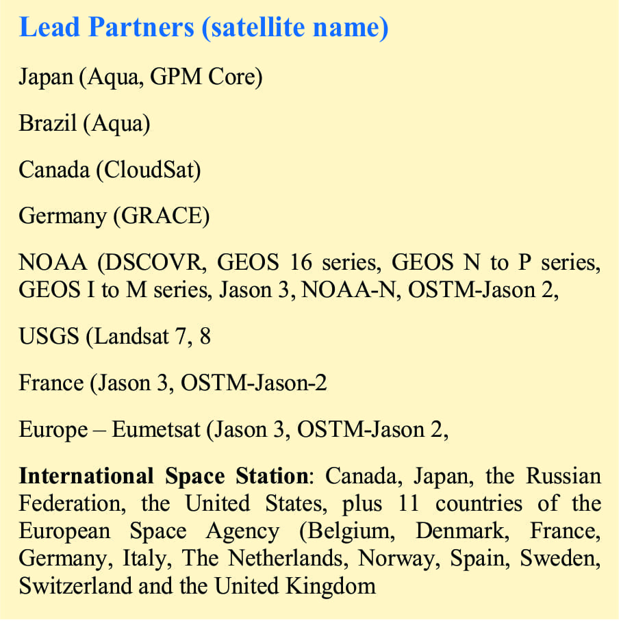
Nine countries have the capability to launch a satellite into orbit (USA, Russia, China, India, France, Japan, Israel, Iran – possibly North Korea). I have focused on NASA and its lead partners because their information is easy to access. However, even this sample shows the breadth of scientific investigation, and the potential for far-reaching advances in global problems such as storm prediction and real-time tsunami monitoring.
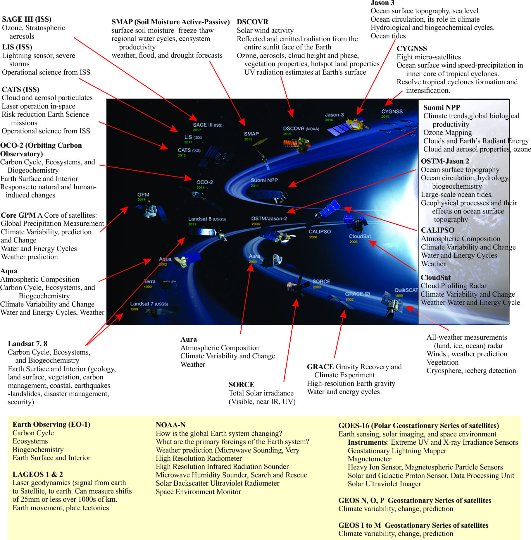
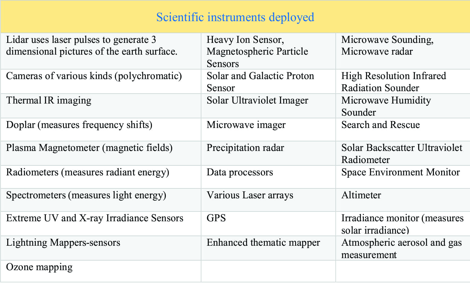
NASA (Earth Observating System) and lead partners Japan, Brazil, Canada, Germany, France, the European Space Agency, and US departments NOAA and USGS, currently have 28 active satellites listed as dedicated to science. The schematic below shows a crude orbital configuration (for 21 satellites) plus the important scientific projects assigned to each satellite. Seven vehicles are listed separately. The instruments responsible for the various data sets are also listed. Some vehicles, like CYGNSS and the GEOS series consist of several small, or micro-satellites. Landsat (USGS), the longest running earth imaging series, began in 1972. The 7th and 8th generation Landsat vehicles are currently operating; a 9th generation satellite is planned for 2020.
The Global Positioning System (GPS) is currently configured from 24 operational satellites.
A wealth of data from measures of our mobile earth, is created every second from these orbiting vehicles. It is the kind of data, not just in its volume, but levels of accuracy and precision, that will justify a rethink of some old theories, and help generate new scientific paradigms about how it all fits together. An optimist would seize the opportunity to develop global and regional-national policies that safeguard the more fragile components of our planet, and mitigate those processes that tend to be less clement. Perhaps it is this inner space, rather than outer-space, that is the final frontier.
Here is a related post on GRACE and LANDSAT