Mohr circles and stress transformation

A montage of stress transformation paraphernalia and rock deformation

Calculating normal stress and shear stress using Mohr circles

Deformation of rock, sediment, and soil is usually manifested as a change in material location, shape, or volume. This means a change in the angular relationship between the original and final configuration of the rock body relative to some coordinate system – in other words, the rock body is rotated. Deformation involves both normal (tension, compression) and shear stresses and as deformation progresses the components of stress must change; in other words, their magnitude and angular relationship to the chosen coordinates changes (note that the ambient stress field is static, at least in the short term). Herein lies one of the more important tasks of structural analysis – calculating the values of the stress components at any stage during deformation. Some of the practical reasons for doing this include:

Determination of the principal stress axes (axes of maximum and minimum stress).
Determining the relationship between normal and shear stress acting on a plane (e.g., an engineered plane, or fault plane).
Calculating the shear stress acting on a body to determine its mechanical stability and potential for failure. This applies to loading or unloading of structural and geotechnical structures such as beams, foundations, bridge spans, the stability of tunnel walls, or soil strength in relation to constructed loads, and to natural surfaces where soil or rock failure can have catastrophic consequences (e.g., earthquakes, slope failures, landslides,).

Transforming the components of stress

The central problem involves calculation of the stress components within a rotating coordinate system. The mathematical expressions we use to calculate the components of stress were developed by the French mathematician-engineer Augustin-Louis Cauchy (1789-1857). The mathematics of continuum mechanics was central to his analysis of the problem. This approach assumes that matter in any material (steel, rock, soil) is continuous – in other words it ignores the real-world condition that most materials, particularly rock or sediment, are composed of discrete particles, grains, or crystals. Thus, the continuum assumes that material is homogeneous (e.g., its composition does not vary throughout) and isotropic – its physical properties, such as density, are continuous in three dimensions. From a mathematical perspective this approach is much simpler than attempting to map all the real- world complexities that exist in Earth materials.

Cauchy began by defining a static 3D structural element within a material body. This element bears no relationship to grains or crystals – it is imaginary. The element is a cube having orthogonal faces that represent the components of normal and shear stress. The element is static which means that the stresses acting on it must balance – this is the initial condition of the element. It exists within a standard Cartesian coordinate system labelled σ_x, σ_y, and σ_{z. (}but note the choice of coordinates is arbitrary).

We can simplify the problem by assuming σ_z is zero and dealing with stress in 2D (the right panel below). Here, σ_x and σ_y can be either tensional or compressional. The element is also subjected to shear stress. Note that the shear vectors τ_xy parallel to the x axis are opposite those parallel to the y axis; this provides the required balance for a static structural element where the shear stresses sum to zero (this does not mean the actual shear stress value along a face is zero).

Cauchy’s 3D and 2D elements and coordinates showing the components of normal and shear stress defined for each face. The coordinates are the standard cartesian system. For a static element, the stresses must balance; this is most easily seen in the 2D element where the shear couples are oriented in opposite directions. Diagrams modified from The Efficient Engineer. — Cauchy’s 3D and 2D elements and coordinates showing the components of normal and shear stress defined for each face. The coordinates are the standard Cartesian system. For a static element, the stresses must balance; this is most easily seen in the 2D element where the shear couples are oriented in opposite directions. Diagrams modified from The Efficient Engineer.

If the 2D element is rotated through an angle θ, the normal and shear stress components will change, as will the coordinates.

Rotation of a 2D structural element through an angle θ and definition of the new stress components. — Rotation of a 2D structural element through an angle θ and definition of the new stress components and coordinates. Calculating the value of these components is central to Cauchy’s method of transformation.

Cauchy developed three equations to solve for the new components σ_x’, σ_y’, and τ_x’y’ for any value of θ (x’ and y’ are the new coordinates) (he did this using some fairly complex maths involving tensor calculus). The solution to these equations assumes we know the values of normal and shear stress in the initial element, i.e., σ_x, σ_y, and τ_xy.

σ_x’ = ½(σ_x + σ_y) + ½( σ_x – σ_y).Cos2θ + τxy.Sin2θ

σ_y’ = ½(σ_x + σ_y) – ½( σ_x – σ_y).Cos2θ – τxy.Sin2θ

τ_x’y’ = – ½( σ_x – σ_y).Sin2θ + τxy.Cos2θ

Cauchy’s three stress transformation equations, where σ_x’, σ_y’, and τ_x’y’are the transformed components of normal and shear stress in the new (rotated) set of coordinates. θ is the rotation angle. Commonly used solutions to calculate the 2θ values are Sin 2θ = 2 Sinθ. Cosθ and Cos 2θ = Cos²θ – Sin²θ.

For more detailed descriptions of stress fields and derivation of the Cauchy transform equations refer to Middleton and Wilcock, 1994, Chapter 4; and Davis and Reynolds, 3^rd Ed. 2012, Chapter 3.

Rotating a structural element through 180^o

We can calculate the normal and shear stress components on a structural element through any angle of rotation using Cauchy’s equations. In the example below, an element is rotated through 180^o at 10^o intervals; the initial and calculated values of σ_x, σ_y, and τ_xy are in units of MPa (megapascals). Plotting the stress values for each σ_x’, σ_y’, and τ_x’y’ against the rotation angle produces sinusoidal curves that contain the following information:

The structural element at 180^o rotation is in the same orientation as at 0^o – extending this through 360^o will repeat the curves.
The maximum and minimum values for each stress can be read directly from the graphs.
The shear stress is zero when the normal stresses are at their maximum and minimum values.
The negative shear stress values refer to reversal of the stress vector directions.

Stress - θ plots of normal and shear stress components for a 2D element, using the initial values for σx, σy, and τxy shown in the left panel. The component values at 180o are the same as those at zero rotation (the initial condition). Maximum and minimum stress values are indicated. The calculations were made using the Civil Engineering Online calculator. — Stress – θ plots of normal and shear stress components for a 2D element, using the initial values for σx, σy, and τxy shown in the left panel. The component values at 180^o are the same as those at zero rotation (the initial condition). Maximum and minimum stress values are indicated. The calculations were made using the **Civil Engineering Online** calculator.

Mohr’s circles

Cauchy’s method for stress calculation is accurate but a bit long-winded (although there are several handy-dandy online calculators that will do the job for you). Otto Mohr (1835-1918) a German engineer-physicist known for his studies on stress and strain, developed a simple graphical system that produces the same results as Cauchy’s equations. Mohr, along with other mathematicians and physicists recognized that the Cauchy equations could be rearranged to express the equation of a circle – having the general form:

(σx – a)² + (σy – b)² = r²

Where a and b are the coordinates of the centre and r is the circle radius.

Stress transformations can be represented by this circle – the eponymous Mohr circle, or Mohr diagram (published in 1882). The Mohr circle contains all the information presented in the graphical plots shown above.

Mohr circle coordinates and angles

The coordinate system used in Mohr’s diagram differs from that used in the element rotation plots shown above; conventionally:

The horizontal axis contains the values for BOTH σ_x and σ_y – σ_x on the right and σ_y the left.
Values of normal stress in tension are positive; in compression negative. Negative values lie to the left of the coordinate origin.
Axes σ_x and σ_y are 90^o apart, but on the Mohr diagram they are plotted 180^o . Thus, all angles on the Mohr circle are twice those of the measured angle of rotation (θ). For example, if θ is 30^o the value on the Mohr circle will be 60^o.
The vertical axis contains values for shear stress τ_xy – positive values below the x-y axis, negative above.
A counterclockwise sense of shear is positive; clockwise is negative (some engineers reverse this convention)
The x-y axis also corresponds to zero shear stress.

Constructing a Mohr circle

We will use the stress conditions for the initial state of the structural element illustrated above but the method applies to any transformed state. The normal and shear stress values on the x and y faces are plotted: (σ_x, τ_xy) and (σ_y, τ_xy). In this example both normal stresses are tensional and have positive values. On the x face, the shear stress τ_xy is positive (counterclockwise sense of rotation) and on the y face it is negative (clockwise).

Note that only the stress components change during rotation – the ambient stress field remains the same.

The x and y faces in the element are orthogonal (90^o) but on the Mohr circle they are 180^o apart. Therefore, the line joining the two points represents a diameter. The circle is drawn on these two points.

Mohr circle drawn for the initial element (green), based on the x face and y face stress values (blue dots). The line between these two points is the circle diameter. Maximum σx and σy values lie on the x-y axis (red dots); Maximum shear stress is read from the tangents to the circle (dashed lines); the horizontal axis represents zero shear stress. Stress values for any value of 2θ can be read on the at any point on the circumference – the actual rotation angle θ is half this value.

The diagram contains the following information:

The values and signs for σ_x, σ_y, and τ_xy for any rotation angle can be read directly from the graph.
In this example, the normal stresses are always positive, and therefore always in tension no matter the rotation angle. However, the shear stress values vary from positive to negative through rotation.
The maximum and minimum values for σ_x, σ_y, and τ_xy are read from tangents drawn parallel to either axis.
The principal stress values σ₁ and σ₂ lie along the line where stress values are zero – this coincides with the x axis.

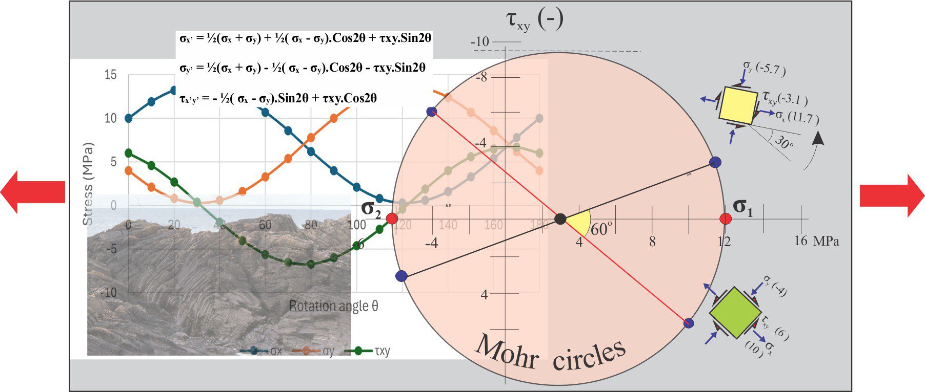
Mohr circle example 2

The initial 2D element in this example (green) has an x-face in tension (positive values) and a y-face in compression (negative values). Plotting the normal and shear stress components for each face gives us two points from which we draw the circle diameter (red line). Note that the circle encroaches on the negative part of the normal stress axis.

Any point on this circle will give us the stress values and signs for the rotation angle relative to the initial element. Examples at 30^o and 60^o rotation are shown. Note that the 2θ angles (60^o and 120^o respectively) are measured from the line (diameter) determined from the initial element.

Mohr plot for an element having positive σx and negative σy. The initial element (green) is rotated counterclockwise 30o (yellow) and 60o (blue). Top right panel shows the rotation data. Maximum and minimum stress values, and the values for the principal stresses σ1 and σ2 (red dots) are highlighted.

Important information contained in the plot:

As with the first example, we can read the maximum and minimum normal and shear stress values and identify the maximum and minimum principal stresses σ₁ and σ₂ respectively (red dots).
Importantly, we can visualize the changes in shear stress as the elements rotate – this is critical data if we are concerned about the stability or potential failure of some structure.
The locus of the y-face normal stress is interesting; initially it is in compression, but during rotation it becomes extensional (blue element).
It is important to remember that these elements are rotating within an ambient stress field that does not change – only the stress components of the elements change.