Stereographic projection – poles to planes

great circles

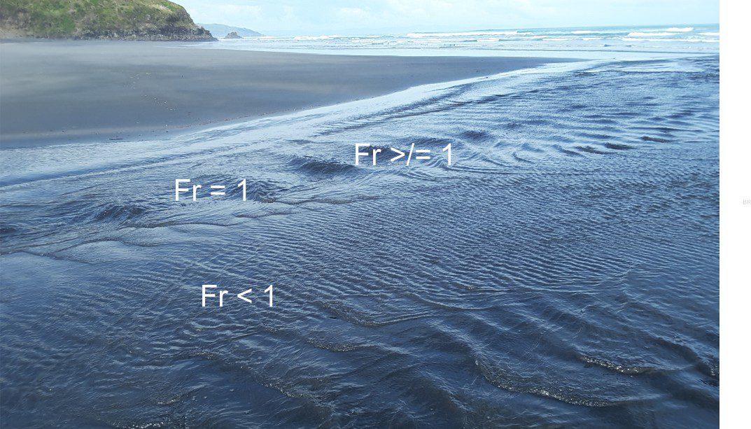
This post is part of the How to… series

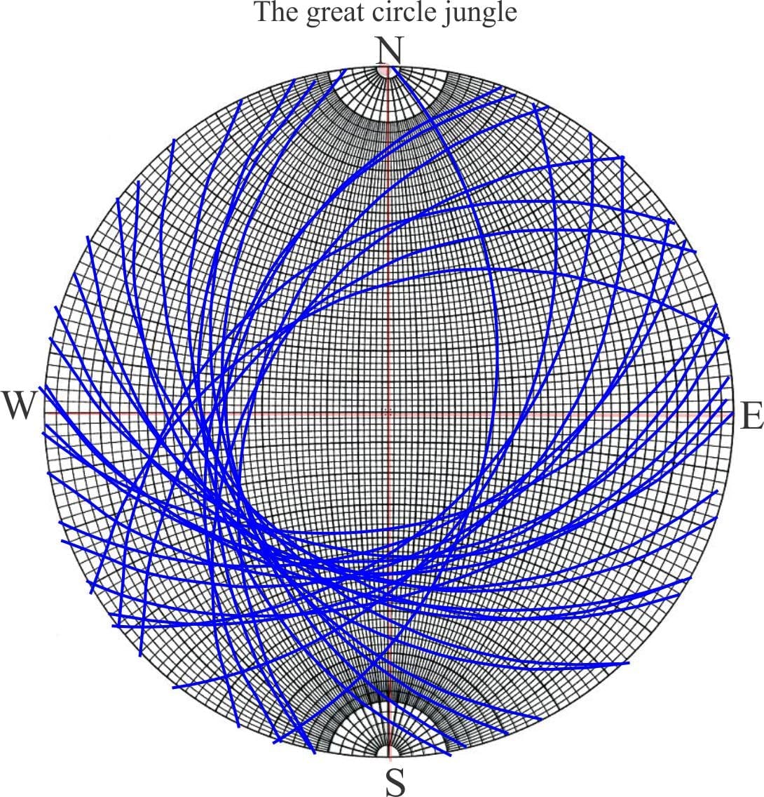
Stereographic projection is used in geology to decipher the complexities of deformed rock by looking at the relationships between planes and linear structures; their bearings (trends) and angular relationships one with the other. The data is plotted on a stereonet as great circles and points (Wulff and Schmidt nets). A stereonet can become pretty messy where there is a lot of data – a seemingly impenetrable maze of great circles. This is where poles-to-planes come into their own.

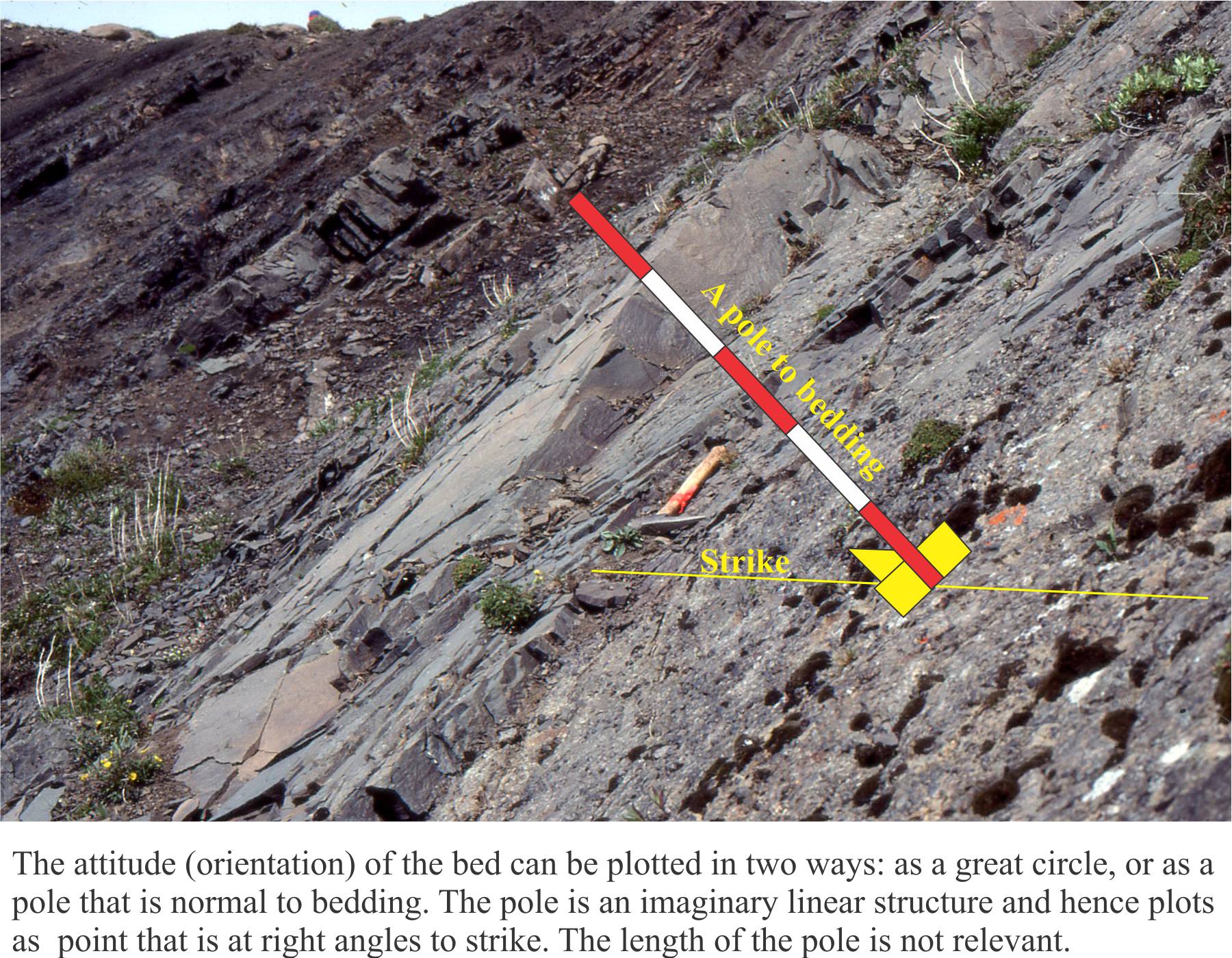
Instead of plotting the great circle to a planar structure like bedding, we plot its pole. Imagine this as a pole oriented at right angles to the plane. Because the pole is a linear feature, it plots as a point on our stereonet. As long as the pole is 90o to strike, it will contain all of the information in the associated great circle. We refer to this point as the pole to bedding (or any other planar feature). Poles to horizontal planes will plot at the centre of the stereonet; poles to vertically dipping planes at the perimeter. Poles to planes dipping at any other angle will plot within these bounds.

Imagine a pole to oriented normal to bedding. The point of intersection on a great circle contains all the information about the attitude of the bed

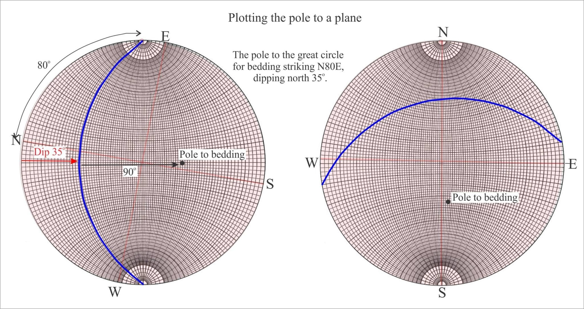
In the example below the orientation of a bedding plane is plotted on an overlay as a great circle. With the great circle pinned to N, count 90 along the W-E axis passing through the centre of the stereonet; this point is the pole.

Plotting poles to bedding no a stereonet

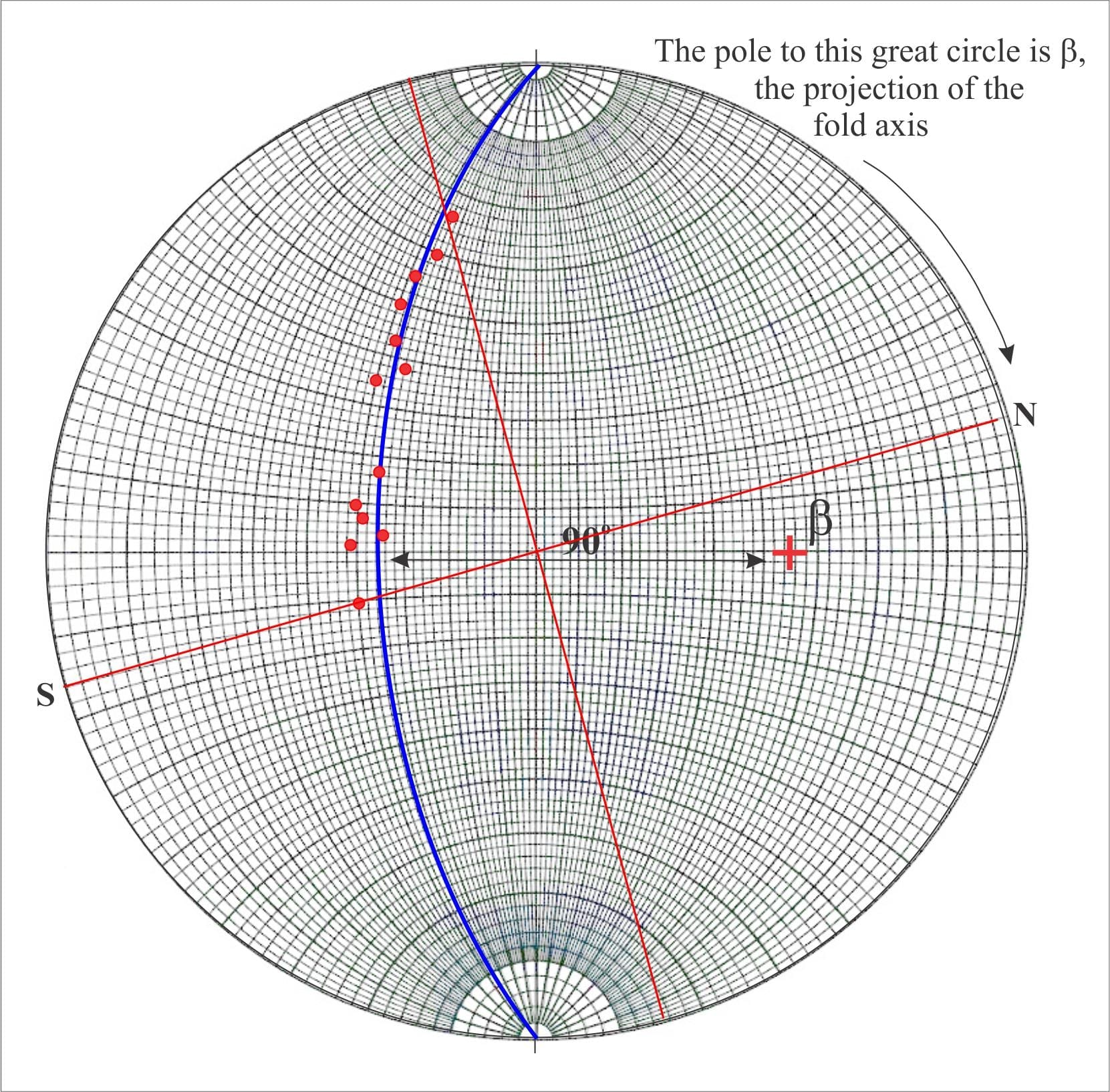
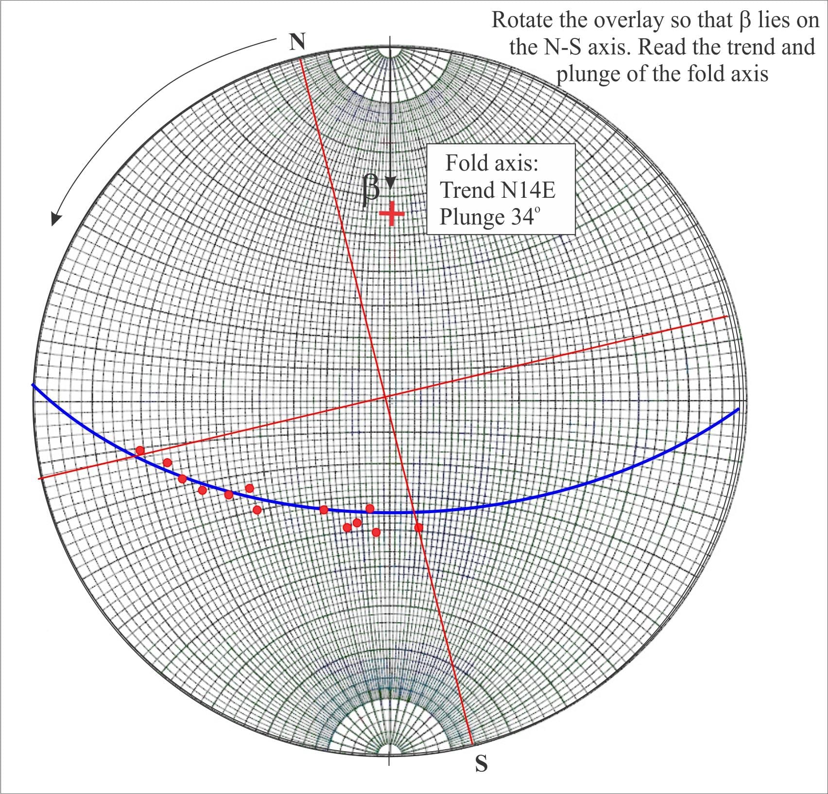
For cylindrical folds the poles to bedding on each limb will all plot on the same great circle (or close to it). The pole to this great circle corresponds to the β point – the fold axis, from which we can read its trend and plunge. Stereographic plots that use poles to bedding or other planes are called pi (π) plots. The utility of pi plots is illustrated in the example of an overturned anticline (the diagrams have been modified from D.M. Ragan, Structural Geology: An introduction of graphical techniques 1968, Figure 11.3).

map of overturned anticline with plotted dips and strikes that can be used to determine the orientation of the axial plane

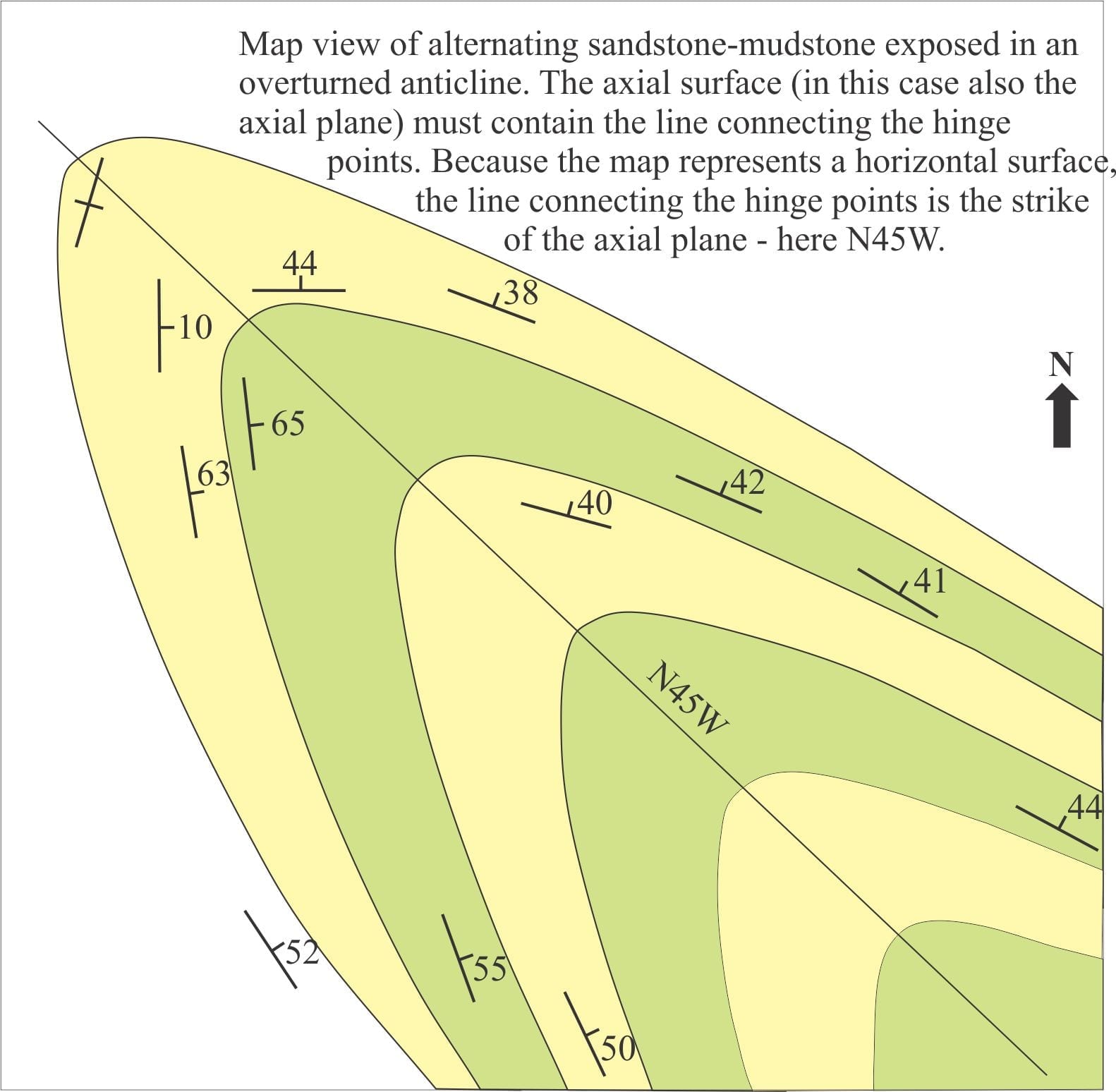
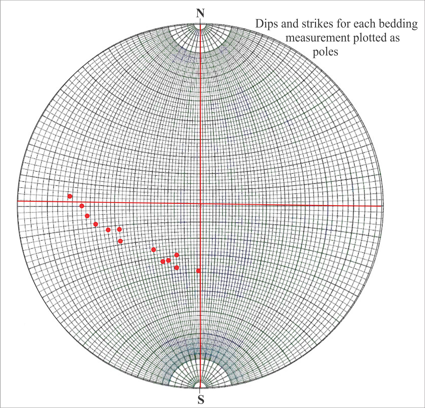
Dip and strike data on each fold limb are plotted as poles to bedding. We can also locate on the geological map the hinge points for each layer. The line connecting hinge points must lie on the axial surface. However, because our map view is horizontal, this line corresponds to the strike of the axial surface – another important piece of information. What we do not know about this structure is the orientation of the fold axis and the dip of the axial plane. The sequence of diagrams that follows shows the main tasks involved in solving this problem.

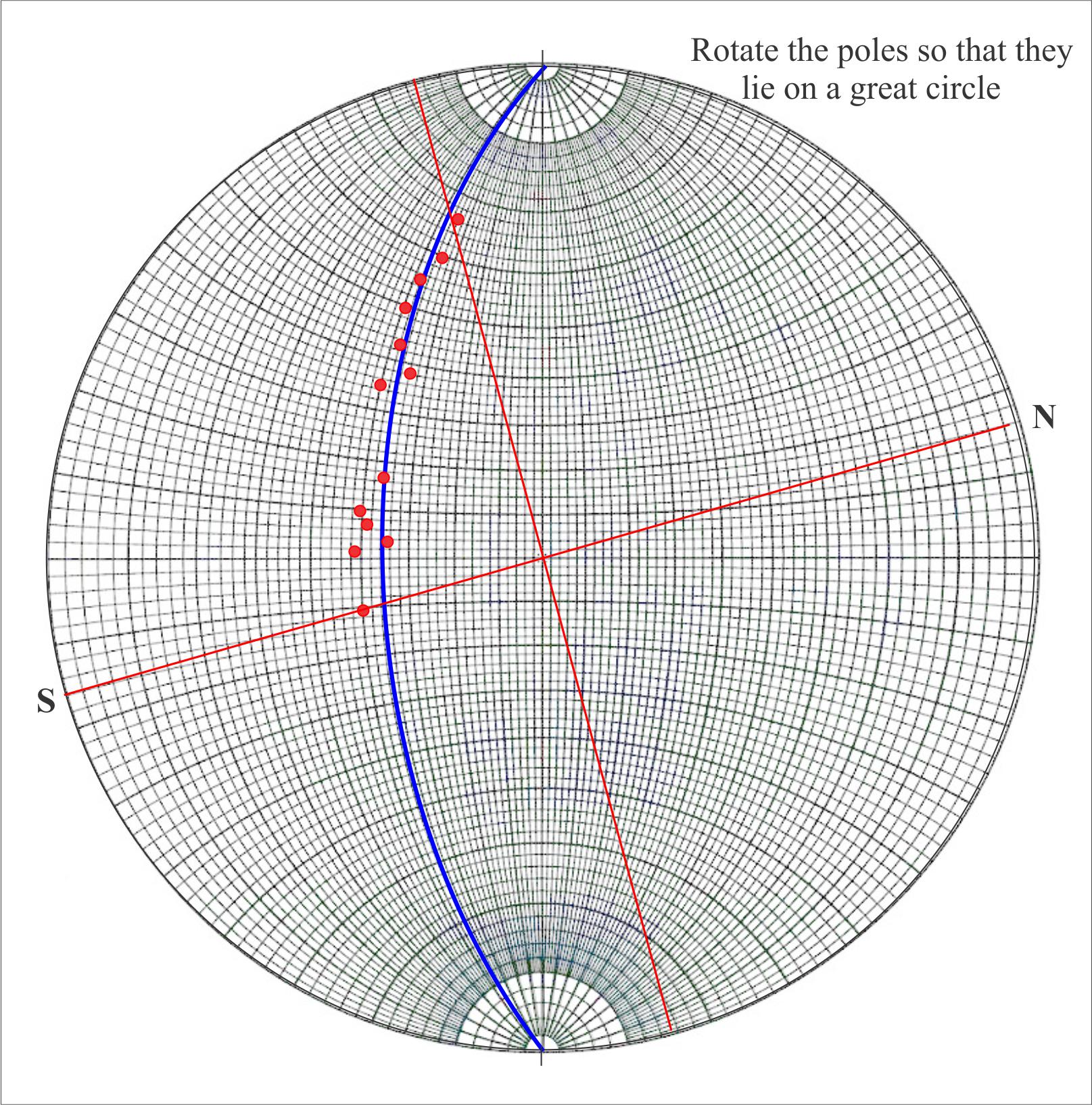
  • Find the great circle describing the poles to bedding by rotating a transparent overlay (make sure you mark the original N-S positions on the overlay).

Dip and strike for each measurement plotted  as poles to bedding                The poles for each bed dip and strike in the fold lie on a great circle

  • With the great circle pinned to North, count 90o from the circle along the east-west axis (the count must pass through the centre of the stereonet); this point is β, the fold axis.
  • Rotate the overlay counter-clockwise until β lies on the N-S axis. From North, read the fold axis trend and plunge.

                Stereographic determination of plunge and trend of the fold axis

Stereographic determination of plunge and trend of the fold axis

  • Plot the line representing the strike of the axial surface (N45W). The great circle containing this line must also pass through β.
  • With the second great circle pinned to North, read the dip of the axial surface.
  • Rotate the completed stereonet back to its original position.
The final plot of fold axis and dip of the axial plane

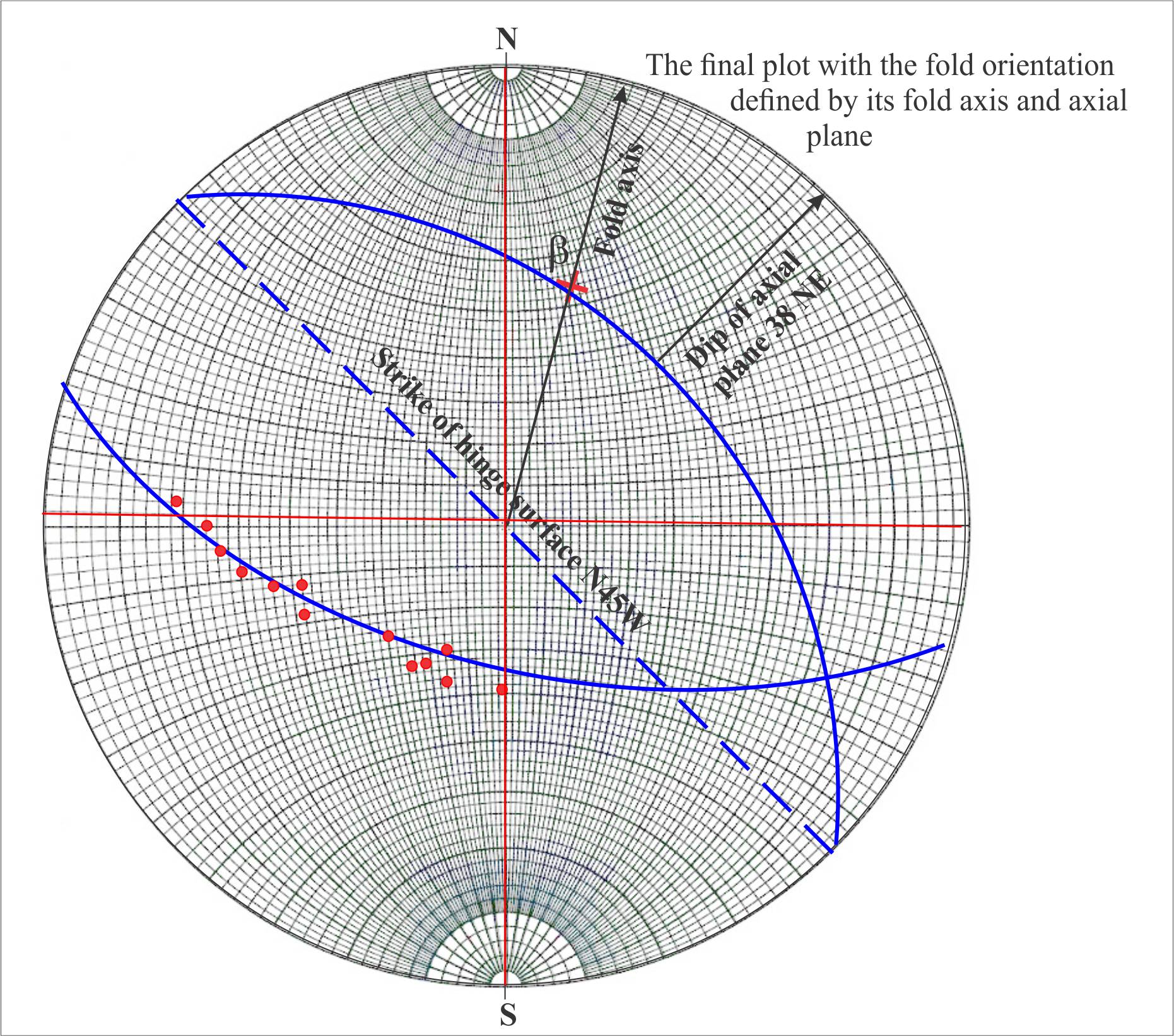
You now have all the information you need to describe the orientation of the anticline.

Some other posts in this series:

Measuring dip and strike

Stereographic projection – the basics

Stereographic projection – unfolding folds

Using S and Z folds to decipher large-scale structures

Leave a Comment

Your email address will not be published. Required fields are marked *

Archives
Categories
Most Popular
Conjugate fractures and en echelon tension gashes – indicators of brittle failure in Old Red Sandstone, Gougane Barra, County Cork, Ireland.
Mohr-Coulomb failure criteria
A montage of stress transformation paraphernalia and rock deformation
Mohr circles and stress transformation
The Marlborough strike-slip fault array extends north from the dextral Alpine Fault transform; faults continue across Cook Strait to join the North Island Dextral Fault Belt in the Wellington region (central Aotearoa New Zealand). In Marlborough and beneath Cook Strait there are several pull-apart basins formed at releasing bend stepovers. Sandbox analogue models can help us decipher the mechanical and kinematic processes that produce structures like these. Base image from NASA – International Space Station 2003.
Strike-slip analogue models
Scaled sand-box experiments are an ideal medium to observe rock deformation that, in this example, involves synkinematic deposition during rift-like crustal extension. The choice of model materials, in addition to imposed boundary conditions such as strain rates, will determine the outcome of the experiment. Dry sand was chosen for this model because its brittle behaviour under the model conditions is a good representation of natural rock failure. Diagram modified slightly from Eisenstadt and Sims, 2005, Figure 3a.
Analogue structure models: Scaling the materials
The relationship between inertial and gravitational forces expressed by the Froude number (Fr) is reflected by the changes in surface flows and the formation-decay of stationary (standing) waves. Fr < 1 reflects subcritical (tranquil) flow; Fr>1 supercritical flow. Although the Froude number can be determined experimentally, it can also be eased out of a dimensional analysis of the relevant hydrodynamic variables.
Model dimensions and dimensional analysis
Recent Posts
Conjugate fractures and en echelon tension gashes – indicators of brittle failure in Old Red Sandstone, Gougane Barra, County Cork, Ireland.
Mohr-Coulomb failure criteria
A montage of stress transformation paraphernalia and rock deformation
Mohr circles and stress transformation
The Marlborough strike-slip fault array extends north from the dextral Alpine Fault transform; faults continue across Cook Strait to join the North Island Dextral Fault Belt in the Wellington region (central Aotearoa New Zealand). In Marlborough and beneath Cook Strait there are several pull-apart basins formed at releasing bend stepovers. Sandbox analogue models can help us decipher the mechanical and kinematic processes that produce structures like these. Base image from NASA – International Space Station 2003.
Strike-slip analogue models
Scaled sand-box experiments are an ideal medium to observe rock deformation that, in this example, involves synkinematic deposition during rift-like crustal extension. The choice of model materials, in addition to imposed boundary conditions such as strain rates, will determine the outcome of the experiment. Dry sand was chosen for this model because its brittle behaviour under the model conditions is a good representation of natural rock failure. Diagram modified slightly from Eisenstadt and Sims, 2005, Figure 3a.
Analogue structure models: Scaling the materials
The relationship between inertial and gravitational forces expressed by the Froude number (Fr) is reflected by the changes in surface flows and the formation-decay of stationary (standing) waves. Fr < 1 reflects subcritical (tranquil) flow; Fr>1 supercritical flow. Although the Froude number can be determined experimentally, it can also be eased out of a dimensional analysis of the relevant hydrodynamic variables.
Model dimensions and dimensional analysis
Scroll to Top