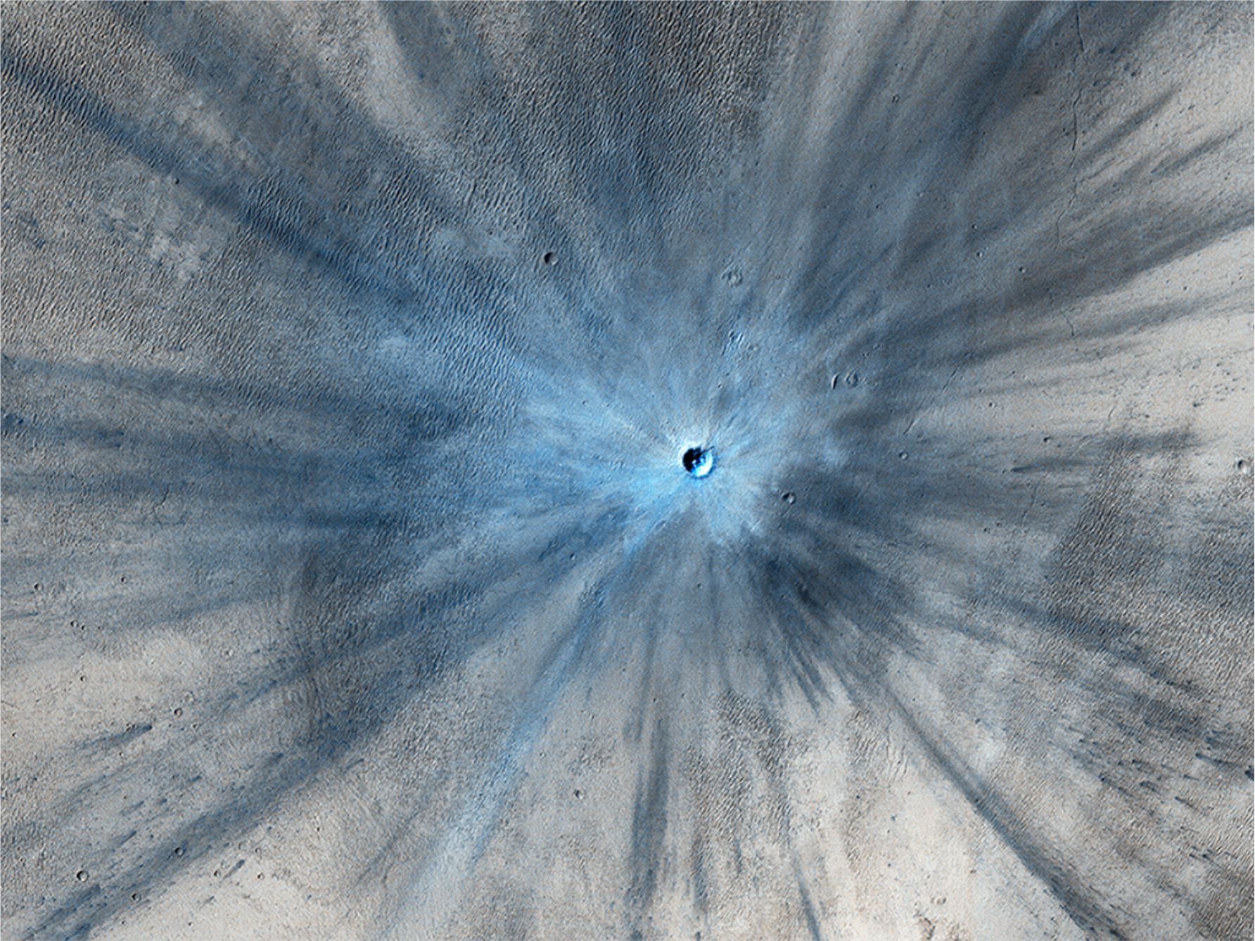
HiRISE has imaged several recent impacts on Mars surface. This one was acquired on November 19, 2013 – images of the site between 2010 and 2012 bracket the impact timing. The crater is 30 m diameter. Impact resulted in a spectacular ray-like zone of ejecta that spreads up to 15 km from the site and partly covers an extensive sand dune field. Image credit: NASA/JPL-Caltech/Univ. of Arizona
The success of the Apollo lunar seismic experiments (1969 to 1977) provided a real boost to Mars exploration. Exploration of the Martian surface began in earnest in the mid-1970s. The Soviet Union had previously attempted to land two vehicles on Mars in 1971 (Mars 2 and Mars 3). Mars 2 crashed; Mars 3 landed successfully but ceased to operate 20 seconds after alighting, without sending any useful information. However, the two Mars orbiters did continue to acquire images for several months.
Mars exploration continued with NASA’s Viking 1 and 2 orbiters that acquired more than 52,000 images of the martian surface. Both Viking landers successfully alighted the surface about 3 months apart in 1976, Viking 1 at Chryse Planitia, and Viking 2 at Utopia Planitia near the margin of the polar ice cap and 6420 km from its cousin. Both landers were able to sample and chemically analyse air and soil (the first time this had been done) and record various weather parameters. The seismometer on Viking 1 failed to operate. That on Viking 2 functioned for 19 months but because it was located on the lander itself the signal to noise ratio was too low to confidently tease marsquakes from wind-generated signals. However, the lessons learned from these and the Apollo missions were successfully applied to Mars InSight experiments 30 years later.
Mars InSight
(The acronym is easier to remember than its full title – Interior Exploration using Seismic Investigations, Geodesy, and Heat Transport).
InSight landed in Elysium Planitia on November 26, 2018, and deployed its seismometer (SEIS) to the martian surface using a robotic arm. Seismic data was recorded until the operation shut down after December 15, 2022 (because dust on the solar panels had reduced their power output).
SEIS recorded events across a broad spectrum of frequencies which means it could record different kinds of seismic events (marsquakes, impacts), but also had to contend with high frequency wind and thermal noise. Thermal noise is generated from heating and cooling of the surface bedrock and regolith, analogous to that found with the Apollo lunar records. However, the experience with seismic noise gained from both Apollo and Viking 2 experiments allowed seismologists to see through these background signals to tease out the lower frequency signals relevant to Mars internal structure. Signal scattering and seismic coda (a kind of echo or ringing) also tend to mask surface waves – these problems were encountered with the Apollo experiments. Like moonquakes, marsquakes are long lived, continuing for 10 minutes and more because of scattering. In fact, the ringing from one event caused by a meteoroid impact lasted several hours.
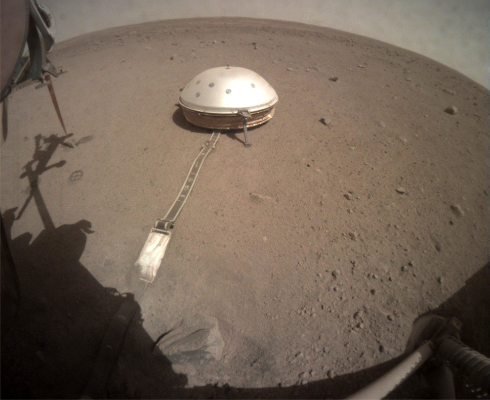
InSight’s seismometer (SEIS) was deployed by a robotic arm to sit directly on the martian regolith. The robotic arm covered the tether with a layer of loose soil to protect it from wind-blown sand and to minimize acoustic noise. The dome also acted as a shield against wind and thermal effects. Dome top is about 80 cm high. SEIS weighed 29.5 kg.
Seismic waves
The symptoms of Earth’s indigestion and hiccups are recorded by seismograms as a succession of seismic wave arrivals. Compressional P waves have the highest velocities and are first to arrive – these are the primary arrivals. They are followed by slower secondary shear or S waves. Both P and S waves are referred to as body waves because they are transmitted at depth through a planetary body; it is these signals that provide most of the information on a planet’s deep internal structure. The time delay between the first P and S arrivals is related to the distance to the quake epicenter.
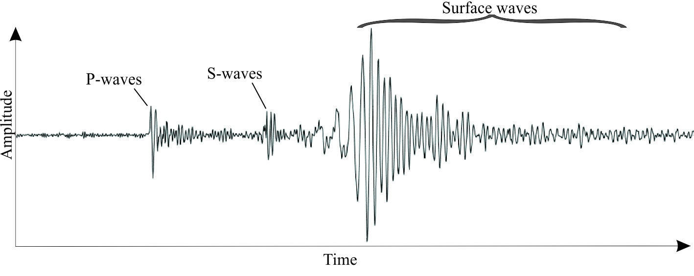
A typical Earthquake seismogram: P-waves arrive first, followed by S-waves. S-waves tend to have lower frequencies than P-waves (more spread out on the graph), but higher amplitude. Surface waves also have the high amplitude and lower frequency than body waves. There can be significant variation on this pattern depending on quake depth, strength, rock composition, and background noise.
P wave deformation is compressional, producing back-and-forth motion at the surface (i.e., motion parallel to the direction of wave propagation). S waves produce up-down and side-to-side motion at the surface (orthogonal to the direction of wave propagation) and tend to be more destructive. S waves are not propagated through fluids (water, gas, igneous melts). Attenuation of S waves at depth in planetary bodies is commonly attributed to a liquid core, or to partial melting in the mantle.
Surface waves confined to the shallow crust comprise a second set of secondary waves that arrive after the body waves (they are slower and have farther to travel). Rayleigh waves produce a rolling ground motion with vertical and horizontal components of movement, and Love waves propagate like S waves but only generate side to side ground movement; they are also attenuated in fluids. Surface waves are most intense following shallow crustal quakes and meteoric impacts; deep quakes produce less intense surface waves.
Marsquakes
More than 1300 marsquakes were recorded over four years of the experiment. Most were of tectonic origin and generated beneath the Martian surface; a few were caused by meteoroid impacts or air bursts. Ninety events having moment magnitudes of 2.5 – 4.2 occurred at teleseismic distances (i.e., distances >1000 km from SEIS).
Two groups of marsquakes have been identified based primarily on frequency: Low frequency (LF) events less than one Hz, and high frequency events (HF) greater than one Hz. HF events are the dominant group and where P and S waves can be identified are attributed to quakes in the crust. LF events usually have recognizable P and S waves and are attributed to deeper quakes. Very high frequency events are mostly caused by thermal responses to diurnal changes in surface temperatures.
Earthquake epicenters can be located accurately because of the large number of seismometers distributed globally. Identifying moonquake epicenters also had the advantage of distributed Apollo seismometer stations. The InSight experiment had only one seismometer such that location of marsquake epicenters required accurate identification of P and S wave arrivals and an a priori seismic model of the martian interior. Note that a general picture of the martian interior (crust, mantle, core) had already been determined from gravity, electromagnetic, and orbital data – what wasn’t known at the beginning of the InSight experiment were accurate depths to the core-mantle-crust boundaries, or the nature of these boundaries.
Signal processing distinguishes between body and surface waves, and between direct P or S waves, and core-reflected and surface-reflected waves. The time delay between P and S waves can be used to estimate to the distance from the epicenter to the seismometer; the same method can also be applied to P and S waves that have been reflected once (designated PP and SS respectively). The modelling process is iterative where both seismic and physical models of the Martian interior are continually updated as the analysis proceeds (for details see Durán et al., 2022, PDF available; and Lognonné et al., 2023, Open Access).
The computed P and S wave velocity-depth profiles are reproduced in the diagram below. Analysis of the low frequency events indicates that their P waves did not traverse deeper than 800 km, much shallower than the expected depth to the core-mantle boundary. S waves on the other hand traversed depths of about 1500 km below which they were strongly attenuated.
However, two notable events in 2021 did produce core-diffracted P waves and surface waves – both were meteoroid impacts (i.e., meteorites or comets) at teleseismic distances from SEIS; both produced large seismic responses with magnitudes >4. The earlier event, S1000a was 7455 km from SEIS and the second event, S1094 was 3460 km (S indicates mission sol, or martian day). Their craters are 130 m and 150 m diameter respectively.
Martian impacts
Six meteoroid impacts or air bursts were recorded by SEIS in 2021, including the S1000a (September 18) and S1094 (December 24) events. Impacts tend to produce relatively strong surface seismic waves, the energy of which depends on impactor size, velocity, and to some extent the obliquity of its trajectory. Two methods of detection and signal analysis have been applied to the martian events:
- Surface impacts and air bursts create a fair bit of noise and atmospheric disturbance that produce above-ground acoustic signals. On Mars, these chirps can be recognized for impacts <300 km from the seismometer – at distances >500 km the acoustic signals are dampened by Mars thin atmosphere.
- Depending in impact size, a mix of body and surface, direct and reflected seismic waves.
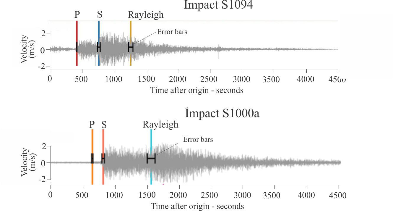
Identification of P and S body waves, and surface Rayleigh waves from the S1094 impact (left) recorded by SEIS December 24, 2021, and S1000a recorded September 18, 2021. Time is in seconds from the first P arrival. Note the long duration post-Rayleigh wave signal run-out to more than 3000 seconds (50 minutes) for S1094 and 3600 seconds (60 minutes) for S1000a. Modified from Posiolova et al 2022 Figures 3 and S1 respectively.
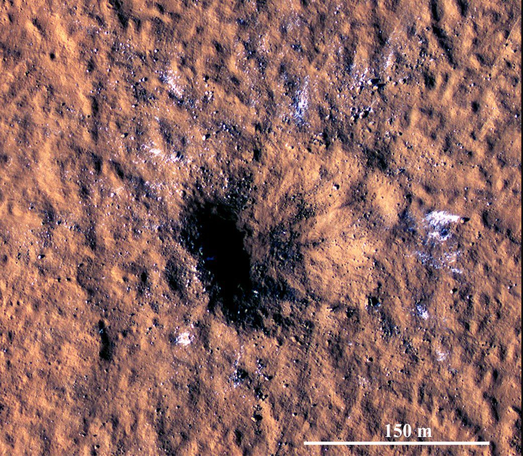
A HiRISE image of the S1094 crater in Amazonis Planitia taken 2-3 Sol after impact. The crater is asymmetric, about 150 m diameter and 21 m deep. Based on empirical models, the impactor was probably 5-12 m across (on Earth it would have burned up on entry). Posiolova et al., (op cit.) calculate the angle of impact at about 30o – the ejecta blanket extends up to 37 km from the crater because of this low angle. White debris in the ejecta is thought to be water ice. Image Credit: NASA/JPL-Caltech/University of Arizona.
The craters from S1000a and S1094 were located by Mars Reconnaissance Orbiter less than 3 Sol after their seismometer recordings (using before and after images of the martian surface). Thus, the impact times and locations are known accurately, providing useful calibrations for marsquake epicenter distance calculations (for example using S-P or SS-PP arrival times). For the two events, the SEIS calculated distance to S1000a was 7591 +/- 1240 km compared with the actual distance of 7461 km; for S1094 the calculated distance is 3530 +/-360 km compared with the measured 3460 km (both differences <1.9%) (Posiolova et al., 2022). The S1094 impact was also notable because it dislodged and scattered blocks of water ice (the bright patches on the image below).
Analysis of the S1000a data indicates P wave diffraction (deflection at a boundary rather than reflection) at a depth between 1500 km and 1600 km (corresponding to a radial distance of 1890-1790 km), that probably corresponds to the core-mantle boundary. The previous P wave depth determined from deep low frequency marsquakes was 800 km (Mars radius is 3,389.5 km measured from the core center).
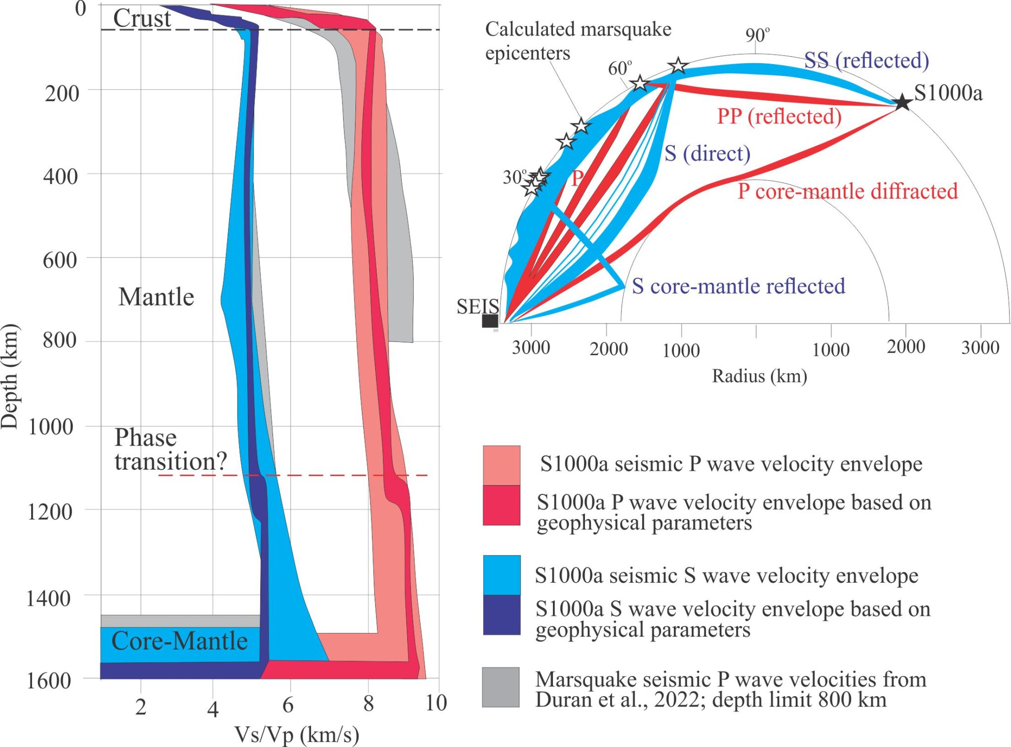
Velocity profiles computed for the S1000a impact show both P and S waves transmitting to 1500-1600 km depth. Light red and blue envelopes include the actual impact seismic data; darker colours define envelopes for velocities calculated from other geophysical parameters. The grey envelopes indicate data from low frequency marsquakes – for these events there are no records of P waves transmitting deeper than 800 m. The ray path map (top right) shows direct (P, S) and reflected (PP, SS) body and surface waves for the S1000a impact and a few low frequency marsquakes. The S1000a P wave was a direct arrival at SEIS although it was diffracted by the core-mantle boundary. Modified from Durán et al., op cit, Figures 3A, 3C.
Mars internal structure: Velocity-depth profiles
Regolith
Data for the upper few decimetres of relatively unconsolidated regolith was generated from impacts used to drive a heat probe into the soil. Conversion of signals indicates seismic velocities for P waves of 0.098 to 0.163 km/s, and for S waves 0.056 to 0.074 km/s through the uppermost 30 cm of regolith beneath InSight (Lognonné et al., op cit).
Crust
Crustal thickness beneath InSight is about 40 km; the base is indicated by an abrupt increase in both P and S wave velocities. Velocity profiles indicate at least two discontinuities within the crust: one at 8-11 km, above which S wave velocities are 1.7 – 2.1 km/s and P wave velocities are 2.5 – 3.3 km/s, corresponding to basalt with 7-10% unfilled porosity (primarily vesicles). The second discontinuity occurs at 20 +/- 5 km. Thus, the data indicates a 3-layered crust. The global Mars average crustal thickness determined from orbital gravity and topography is 30-72 km Lognonné et al., op cit).
Core-Mantle
The conclusion that Mars core is iron-rich is based primarily on bulk density, gravity and orbital data. Various geophysical, seismic, orbital moments models have been used to calculate the core radius and core-mantle boundary (discussed in some detail by Lognonné et al., op cit). There is reasonable consensus that the core-mantle boundary is between 1,500 and 1,600 km depth, corresponding to a core radius of 1,890-1,790 km. P waves from meteoroid impacts S1000a and S1094 confirm this boundary depth, a depth that also corresponds to significant attenuation of shear (S) waves.
There is a P and S wave discontinuity at about 1,100 km depth that may correspond to a mantle mineral phase transition and an increase in mantle density. This boundary may be analogous to mineral phase – density transitions determined for Earth’s mantle, for example in olivine or perovskite (also common minerals in chondritic meteorites). Average core density is about 6,000 – 6,300 kg/km3.
There is still debate about the structural aspects of Mars’ core. Does it have a solid inner core and molten outer core (S wave behaviour indicates likely melting at the core-mantle boundary) or is the entire core liquid? Le Maistre et al., (2023) argue the latter based on detailed measurement of Mars rotation using InSight RISE data (Rotation and Interior Structure Experiment), demonstrating a rotational wobble that is best explained by a liquid core. The core radius in their calculations is 1,835 ± 55 km, and the bulk density is 5,955–6,290 kg m−3 corresponding closely to the values obtained from seismic and other geophysical data.
Unlike Earth, there is no evidence for rotation of Mars outer core. As a consequence, Mars has no geomagnetic field to shield it from solar and cosmic radiation. Given the almost overwhelming sedimentary and geochemical evidence for ancient seas and lakes on Mars surface, Mars atmosphere must have been significantly denser than at present (Mars present atmospheric pressure is less than 1% of Earth’s at sea level) and it is likely that core conditions were very different in the past. Stripping of Mars’ atmosphere by solar winds was probably a direct result of the slow down of core rotation and consequent loss of its geomagnetic shield.
Other posts on planetary geology
A measure of the universe: Renaissance slide-rules and heavenly spheres
Comets; portents of doom or icy bits of space jetsam?
Sand dunes but no beach; A Martian breeze
A watery Mars: Canals, a duped radio audience, and geological excursions
Which satellite is that? What does it measure?
Life on Mars; what are we searching for?
Io; Zeus’s fancy and Jupiter’s moon
The origin of life; Panspermia, meteorites, and a bit of luck
Near Earth Objects; the database designed to save humanity
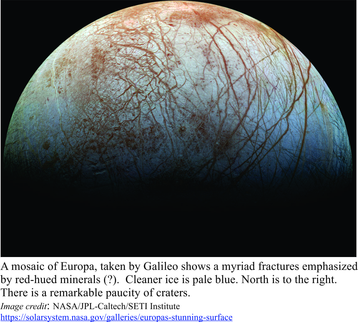
Subcutaneous oceans on distant moons; Enceladus and Europa
Visualizing Mars landscape in 3 dimensions; stunning images from HiRISE
Martian organics; One more step in the right direction
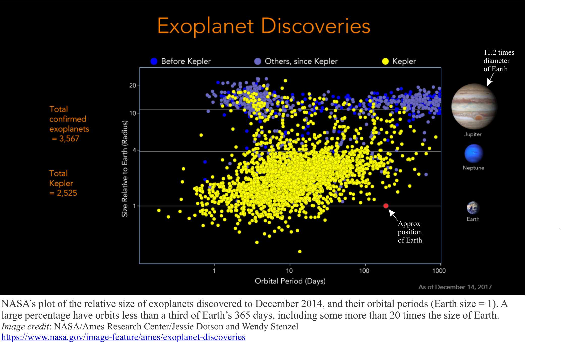
There are more exoplanets than stars in the universe
Archeomagnetic jerks: Our decaying magnetic field
Seismic experiments and moonquakes