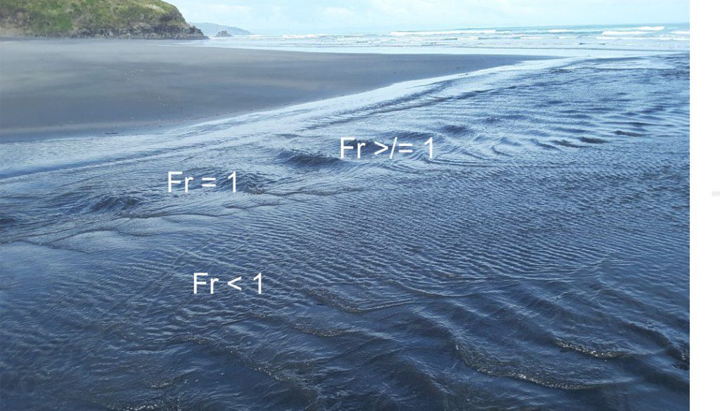
Model dimensions and dimensional analysis

The relationship between inertial and gravitational forces expressed by the Froude number (Fr) is reflected by the changes in surface flows and the formation-decay of stationary (standing) waves. Fr < 1 reflects subcritical (tranquil) flow; Fr>1 supercritical flow. Although the Froude number can be determined experimentally, it can also be eased out of a dimensional analysis of the relevant hydrodynamic variables. — The relationship between inertial and gravitational forces expressed by the Froude number (Fr) is reflected by the changes in surface flows and the formation-decay of stationary (standing) waves. Fr < 1 reflects subcritical (tranquil) flow; Fr>1 supercritical flow. Although the Froude number can be determined experimentally, it can also be teased out of a dimensional analysis of the relevant hydrodynamic variables.

The correct scaling of geometric, dynamic, and kinematic system variables is a critical part of any useful analogue model.

Most physical systems operate with a multitude of variables. The interplay amongst these variables is complicated. System models help us organize the various processes and responses in a way that gives us some understanding about how the systems work. The modeling process itself requires us to reduce the number of variables to some manageable level. Dimensional analysis identifies the important groups of variables and, according to the rules of algebra, express these relationships as equations. Dimensional analysis can help us discover new relationships (as equations) or, if the equations are known a priori, help check their validity.

In any discussion of physical processes there will be inevitable reference to measurable or theoretical quantities such as volume, acceleration, or force. Each of these quantities, or variables has two properties that are independent of their actual numerical values:

Units of measure that comply with some recognised system, such as metric (centimetres, grams), imperial (feet, pounds), SI (metres, kilograms) or Babylonian (cubits), and
Fundamental dimensions that for most dynamical and mechanical systems includes mass [M], length [L], and time [T]. In some cases, force [F] may be used instead of mass because it is a combination of all three dimensions. Systems that involve other physical or chemical parameters include dimensions like temperature and electrical charge in this list. For our discussion, the [MLT] triad will suffice.

The standard presentation of dimensions is to enclose them in square brackets [ ]. The variables most commonly used in dynamic and kinematic problems include:

Length l [L] (e.g., depth, distance, grain diameter)

Area A [L²]

Volume V [L³] (NB. If we define a volume cross-section as unit area, V can be expressed as height or depth [L]

Mass m [M]

Time t [T]

Specific weight γ = ρg [ML^-2T^-2]

Density ρ = m/V [ML^-3]

Velocity v = l/t, or dx/dt [LT^-1]

Acceleration a = l/t² [LT^-2]

Force F = ma [MLT^-2]

Pressure/stress P = F/A [ML^-1T^-2]

Momentum p = mv [MLT^-1]

Viscosity the coefficient μ in the function μ.dV/dl [ML^-1T^-1]

Some rules and advantages governing dimensional analysis

Dimensional homogeneity: This applies to equations, where the dimensions must be the same on either side of the equality. This condition was probably first stated by French mathematician Jean-Baptiste Fourier (1768-1830). In a standard algebraic equation, each term must have the same dimensions. For example, the equation of a straight line y = mx + c where gradient m is dimensionless [L/L], and x, c both have dimensions [L], therefore y must also have the dimensions [L].
The dimensions of the numerator and denominator in a ratio must be the same.
Dimensional integrity must be maintained when converting a variable from one unit system to another system. For example, the SI unit of pressure is the Pascal (Pa) expressed as kg/m.s² [ML^-1T^-2], and the imperial unit is pound force/square inch, or force per unit area – with dimensions [MLT^-2].L^-2, or [ML^-1T^-2].
Some quantities are dimensionless. Angular quantities like degrees and radians have no dimensions – they are numbers. All ratios are dimensionless – porosity is a ratio of volumes, physical strain is a ratio of lengths or volumes.
Dimensional analysis gives us a logical way to scale experiments on real world systems and processes in a way that allows us to answer questions about how things work.

The Buckingham pi () theorem

Newton’s laws are fundamentally empirical and expressed in mathematical form as equations. Newton and his contemporaries must have considered the concept of dimensions given the paramount importance of these equalities. However, the utility of dimensional analysis is a relatively modern advance, first encouraged by the British physicist Baron Rayleigh and others in the late 19^th C (Bramwell, 2017). The rules of dimensional analysis and scaling are encapsulated in the Buckingham pi theorem. Formal definition of the pi theorem as a set of algebraic rules is attributed to American physicist Edgar Buckingham (On physically similar systems: Illustrations of the use of dimensional equations, The Physical Review Ser.2 v.3-4, 1914), although some of his predecessors, like Joseph Bertrand may have formulated the procedure as early as 1878. The theorem provides a mathematical method for simplifying the number of variables in a system, so that the system analysis is manageable. The method is an important part of analogue modeling.

The pi theorem is a procedure for identifying dimensionless groups, or products from the system variables. A more formal statement is commonly quoted thus: If there are x variables in a problem and these variables contain y primary dimensions, the algebraic function relating all the variables will have (x-y) dimensionless groups (a procedure also known cumbersomely as nondimensionalization). Each group is a ratio consisting of two or more variables. Buckingham named these pi groups (π1, π2, π3… not to be conflated with the quantity pi). One of the primary goals of dimensional analysis is to establish these pi groups, the procedure for which is best illustrated by an example.

The example of fluid flow through a pipe

We want to derive an expression for the pressure drop that enables fluid flow through a straight pipe. This is a classic problem that in the late 19^th C led to an important discovery.

The pipe is straight, with circular cross-section of diameter D. We simplify the problem by assuming the inside of the pipe is smooth (so we don’t have to account for surface roughness). There is a pressure drop (ΔP) over a length l.

We first identify the relevant system variables and their dimensions: D [L], l [L], ΔP [ML^-1T^-2], mean velocity v [LT^-1], fluid density ρ [ML^-3], and fluid viscosity μ [ML^-1T^-1].
We can write the general function for this system as f(D,l, ΔP,v,ρ,μ) = 0
The list contains 6 variables and 3 dimensions. According to the pi theorem (x_variables – y_dimensions) there are three dimensionless groups (π1, π2, π3). From the list of variables, we need to identify three that are independent (because we have three dimensions) – such quantities are called repeating variables – repeating variables have dimensions. Independence here means that each variable must not be a multiple or power product of others in the set (e.g., the square or square root). Middleton and Wilcock (1974) also advise that we should not chose variables that are of most interest to the problem – in this case we should not chose ΔP as an independent variable because we want to determine what it is actually dependent on. For example, if we choose D, v, and ρ, the possible combinations (like D/v, ρ/D or v/ρ) do not produce dimensionless quantities. Therefore, all three variables are independent of each other. Note we cannot choose both D and l because the ratio of these two variables will always be dimensionless.
As noted above, the system we have defined has three possible dimensionless groups. To find the dimensionless groups, we need to combine the three independent variables with each of the remaining variables ΔP, l, and μ in turn. For the first pi group we try

D, v, ρ and ΔP.

Note that the dimensions of any quantities have exponents. For nondimensionality to apply, the sum of the exponents of each dimension (M, L, and T) must be zero. To evaluate the pi groups, we need to assign exponents to the dimensions of each independent variable (exponents a, b, c); we arbitrarily assign the exponent of the dependent variables as 1.

The first pi group is written as:

π1 = D^a v^b ρ^c ΔP¹ that, expressed as dimensions is:

π1 = [L]^a [LT^-1]^b [ML^-3]^c [ML^-1T^-2]¹

We can now write three algebraic equations that sum the exponents of each dimension in this pi group (each must sum to zero):

For M c + 1 = 0

For L a + b -3c -1 = 0

For T -b -2 = 0

Solving, c = -1, b = -2, a = 0 (π1 does not contain an L dimension).

We can now write the π1 in terms of actual exponents:

π1 = [LT^-1]^-2 [ML^-3]^-1 [ML^-1T^-2]¹ that, in terms of the variables is

π1 = ΔP/ρ v²

We perform the same calculations for π2 and π3 and get:

π2 = μ/ρvD and

π3 = L/D

We can now rewrite the general function for the system as f₂(π1,π2,π3) = 0, that expressed as variables and rearranged is:

⸫ ΔP/ρ v² = f₂(μ/ρvD, L/D) which states that the pressure drop is a function of π2 and π3.

π2 is usually inverted and becomes ρvD/μ which is the Reynold’s number.

Thus, the pressure drop in the pipe is a function of the Reynold’s number and the ratio of its length to its diameter.

Dimensional analysis has not only answered the question about the fluid flow pressure drop, it is also capable of generating and verifying important dimensionless quantities such as Reynolds’, Froude, and Stokes numbers.