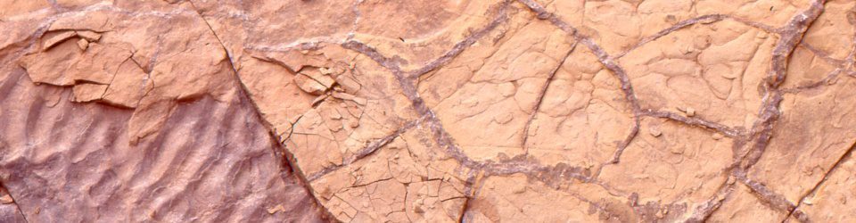
The cyclic repetition of conglomerate beds (resistant units) and interbedded (recessive) shales resulted in a 700+ m-thick stack of fan deltas, where sediment accommodation was generated in the foot wall of an active reverse fault ( Jurassic, northern British Columbia). The near vertical dips resulted from later thrust faulting and folding. Stratigraphic top to the right.
Stratigraphic repetition, stratigraphic cycles, and stratigraphic trends
We know with reasonable certainty that the sun will rise tomorrow. We know this because it has taken place every day for the last 4.6 billion years. The repetition of this event is comforting; it adds symmetry to our lives – it is predictable.
The universe is full of repeatable events and processes, from the birth and death of stars to the spin of an electron. Some events occur in a more or less haphazard way, with little sense of regularity, or periodicity. Volcanic eruptions are notoriously difficult to predict – any periodicity, if it exists, has alluded our concerted efforts to decipher it. Other events are remarkably regular in their occurrence: night follows day, the ebb and flood of tides, sunspot maxima to minima.
We refer to the regular repetition of events as cycles. Cycles have periodicity – the time it takes to complete one revolution (completion of Earth’s orbit around the sun), or the passage of a wave. The period of sea or lake surface waves is the time it takes one wave crest (or trough) to the next crest to pass a reference point; surface wave periods are measured in seconds. Milankovitch (astronomical) orbital cycles have periodicities measured in 104 to 105 years. One of geology’s grandest cycles is the Wilson Cycle that describes the birth and death of ocean basins over 180-200 million years.
We also recognise cycles in stratigraphy, recorded in the repetition of sedimentary facies, fauna and flora associations, sediment chemistry, and hiatuses or discordant surfaces, that all represent changing depositional environments over time, fluctuations in relative sea level and sediment accommodation, migrating shorelines, and the changing conditions of sediment storage and release. Stratigraphic cycles are known from almost all depositional environments on Earth – terrestrial to deep marine; some are 10s of metres thick, others a few millimetres. All these cycles have periodicities, although measuring them continues to be a problem for stratigraphers, particularly those of durations less than the resolution of biostratigraphic or radiometric measures of age.
An example from the Jurassic of northern British Columbia
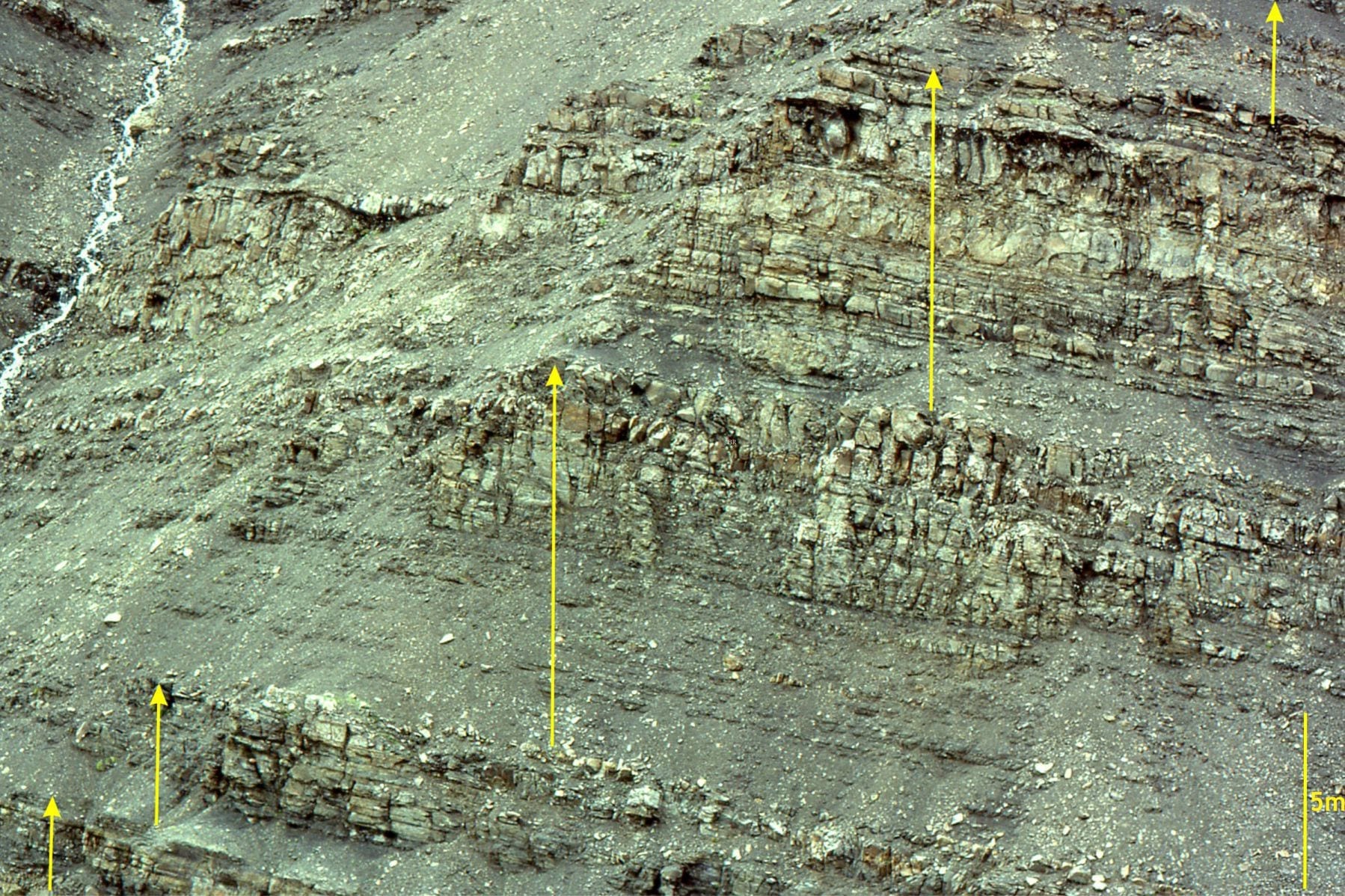
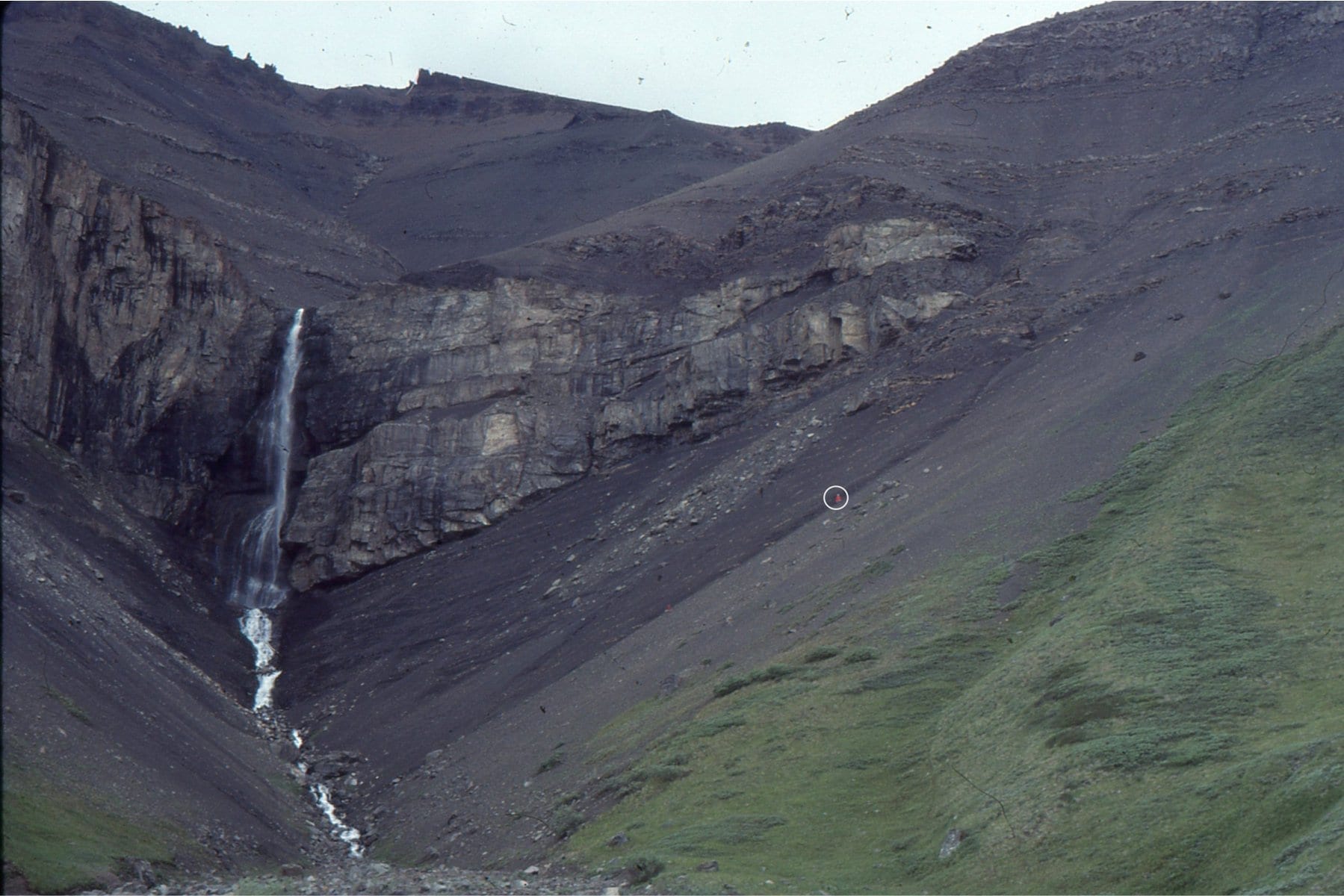
Packages, or cycles of shale through sandstone, each a few metres thick, are repeated 5 times over about 35m in this outcrop view. Arrows indicate the base and top of each cycle. The example is from Bowser Basin, northern British Columbia.
The outcrop image shows the repetition of shale and sandstone beds over a stratigraphic thickness of about 35m. Working through the outcrop, we observe the following sedimentary and stratigraphic associations:
- Each package of grey, laminated mudstone, siltstone and thin, ripple-bedded sandstones (2-3m thick), abruptly overlies thick sandstones. Fossils include ammonites, trigonid bivalves, and Buchia, all indicative of an open marine environment.
- For each package, working our way upward, the proportion and thickness of sandstone beds increases; the upper 1-2m are predominately sandstone.
- With the increase in the proportion of sandstone beds is a concomitant increase in grain size, from fine-grained to coarse-grained sandstone at the top.
- The size and frequency of crossbeds increases upwards.
The pattern of facies, from mudstone to sandstone, is repeated five times in this outcrop view, and in fact is repeated dozens of times through the remainder of the exposure. We recognize this stratigraphic repetition as cyclical. The cycles are 5-20m thick. In each cycle there is a reasonably consistent change in grain size from bottom to top – we refer to this stratigraphic trend as coarsening-upward (a descriptive term).
For each cycle, the vertical transition in facies is interpreted as a change from relatively low energy, outer shelf (the mudstone facies), to higher energy inner shelf where wave and current action move sediment (crossbedded sandstone facies). Based on the interpretations, we refer to this kind of stratigraphic trend as shallowing upward (a genetic term).
We designate the base of each cycle at the abrupt contact between mudstone-shale and the underlying sandstone; the rationale for this is:
- It is easily identified and is mappable,
- It is consistent from one cycle to the next, and
- It signals an abrupt change in depositional environment – from relatively shallow shelf (shoreface), to deeper outer shelf. The contact thus represents a significant change in relative sea level (in this case a transgression).
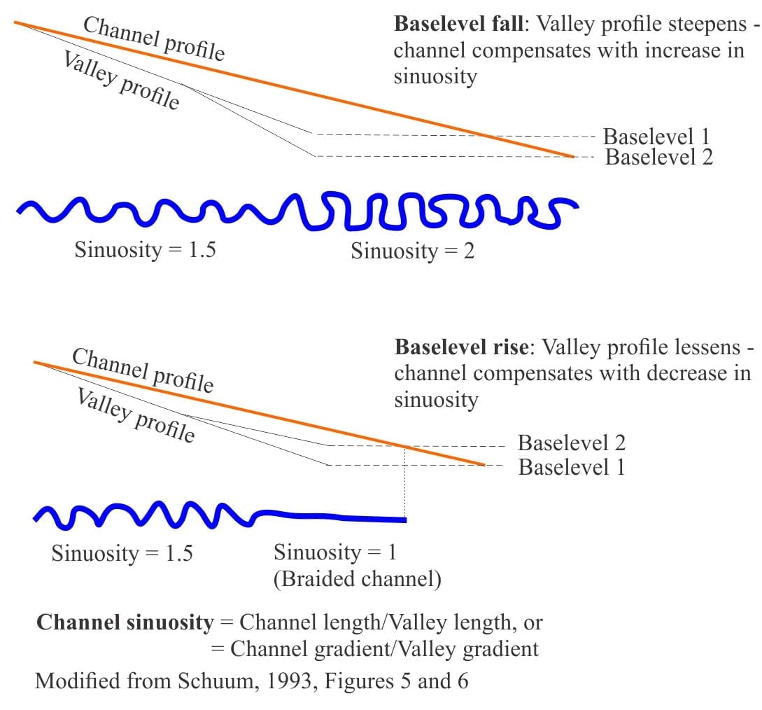
Coarsening-shallowing upward cycles are common in marine successions that are subjected to fluctuating baselevels, sediment accommodation and the seaward or landward migration of shorelines. The opposite trend, fining upward cycles are also common, particularly in fluvial systems; the classic meandering (high sinuosity) channel and point bar cycle contains trough crossbedded sandstone at its base, fining upward to mud-silt-coal facies deposited on floodplains. In this case, the cycles represent changes in channel baselevel, depositional slope, and storage or release of sediment.
Cycle hierarchies
Five hundred years and more of stratigraphic analysis has shown us that there is a hierarchy of cycles that we tend to equate with changes in baselevel,
typically relative sea level. We presently recognize:
1st order cycles – about 50-100 Ma; Continent-wide sequences that represent tectonic plate reorganization such as the break-up of Pangea and Gondwana, and protracted events like the opening of Atlantic Ocean. Commonly cited examples include the Absaroka, Tippecanoe, and Sauk Sequences of North America.
2nd order cycles – about 5-50 Ma; Superimposed on 1st-order cycles, they may represent changes in mid-ocean ridge spreading rates. 1st and 2nd-order sea level fluctuations are controlled by tectonic, isostatic, and thermal processes (e.g. thermal cooling following a rift episode), as well as glacio-eustatic and climate variations.
3rd order cycles – about 0.2-5 Ma; There is no single mechanism that controls these brief excursions in relative sea level, but probably includes some short-lived plate reorganizations, the isostatic response to tectonic loading and unloading (particularly at convergent plate boundaries), and glacio-eustatic episodes. Sea level fluctuations are measured in 10s of metres. Note that 3rd-order cycles generally coincide with 3rd-order stratigraphic sequences in the original Vail-Exxon Sequence Stratigraphy model.
4th order cycles – about 100-200 thousand years (ka); Sea level excursions are measured in metres to perhaps 20m (see notes below)
5th order cycles – 10 years -100 ka; As for 4th-order cycles, sea level excursions are measured in metres to perhaps 20m. Although local tectonics may play some role in these short-duration cycles, the primary controls on sea level are thought to be caused by thermal (steric) and glaciation-deglaciation changes to ocean volumes. These short-term fluctuations have periodicities coincident with changes in solar insolation (a measure of the incident radiation reaching Earth), that varies according to Milankovitch orbital cycles: Eccentricity cycles (about 100 ka), Obliquity cycles (41 ka), and Precession cycles (22 ka). Milankovitch orbital cycles are commonly invoked as controls on high order stratigraphic cycles – an hypothesis worthy of debate. These controls on baselevel (sea level) are external to most 4th-5th order depositional systems (i.e. they are allogenic). We now know that autogenic processes can produce cycles at these periodicities. Thus, it is important when analysing 4th and 5th order cycles to take into account the relative contributions of autogenic sedimentation dynamics.
Each cycle order does not occur on its own, independent of the other cycles. Think of them as nested, for example where 2nd-order cycles are superimposed on 1st-order, 3rd-order on 2nd-order, and so on. A useful analogy to help visualize these interactions is the interference of surface waves propagated in different direction; the interference may be destructive or constructive. Thus, a 4th-order sea-level rise that is superimposed on a 3rd-order sea-level fall, will tend to decrease the rate of fall, or even create a temporary rise in the 3rd-order trend. One of the first geologists to consider quantitatively the interactions among the cycle hierarchy was Joseph Barrell (1917).
The Jurassic example again
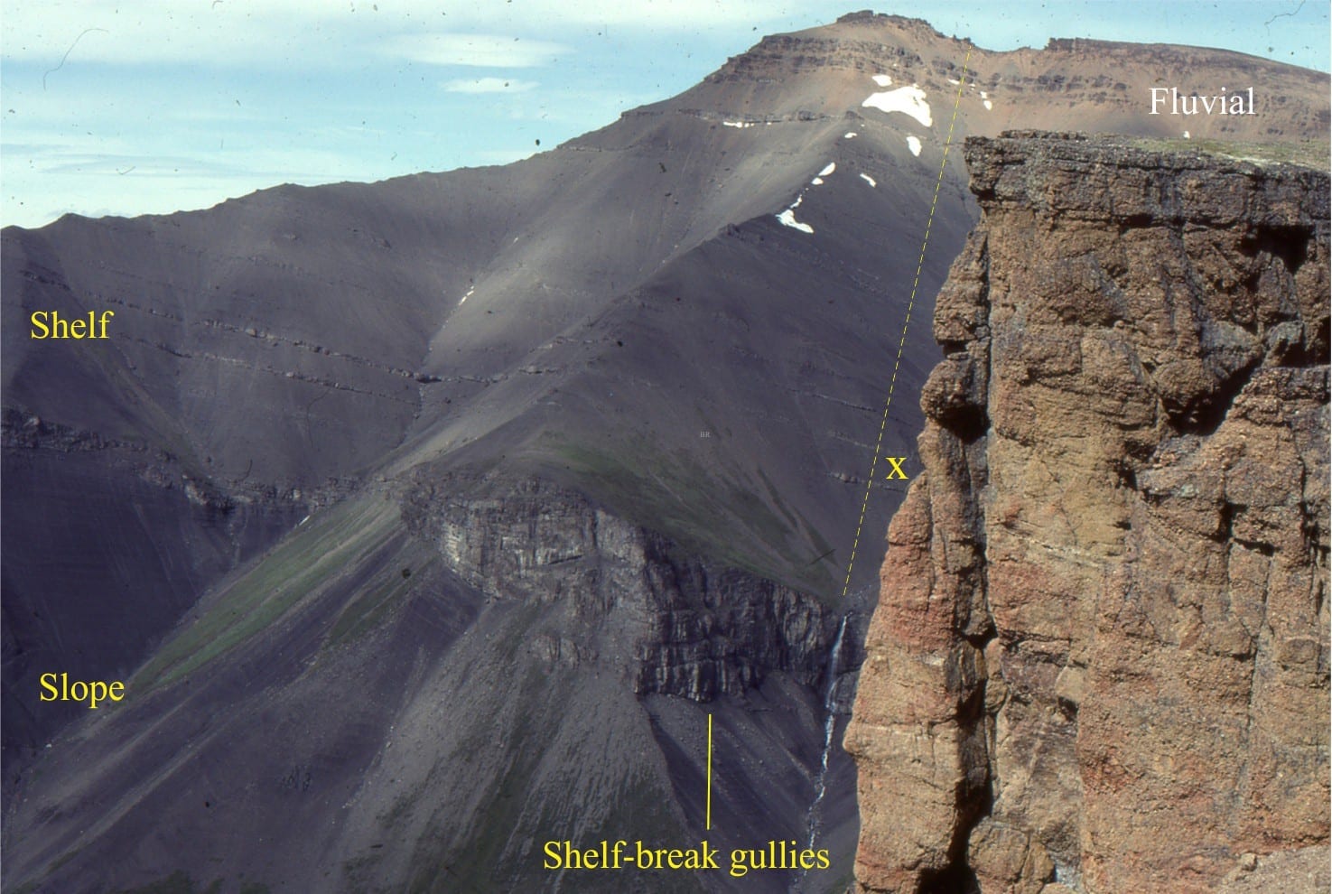
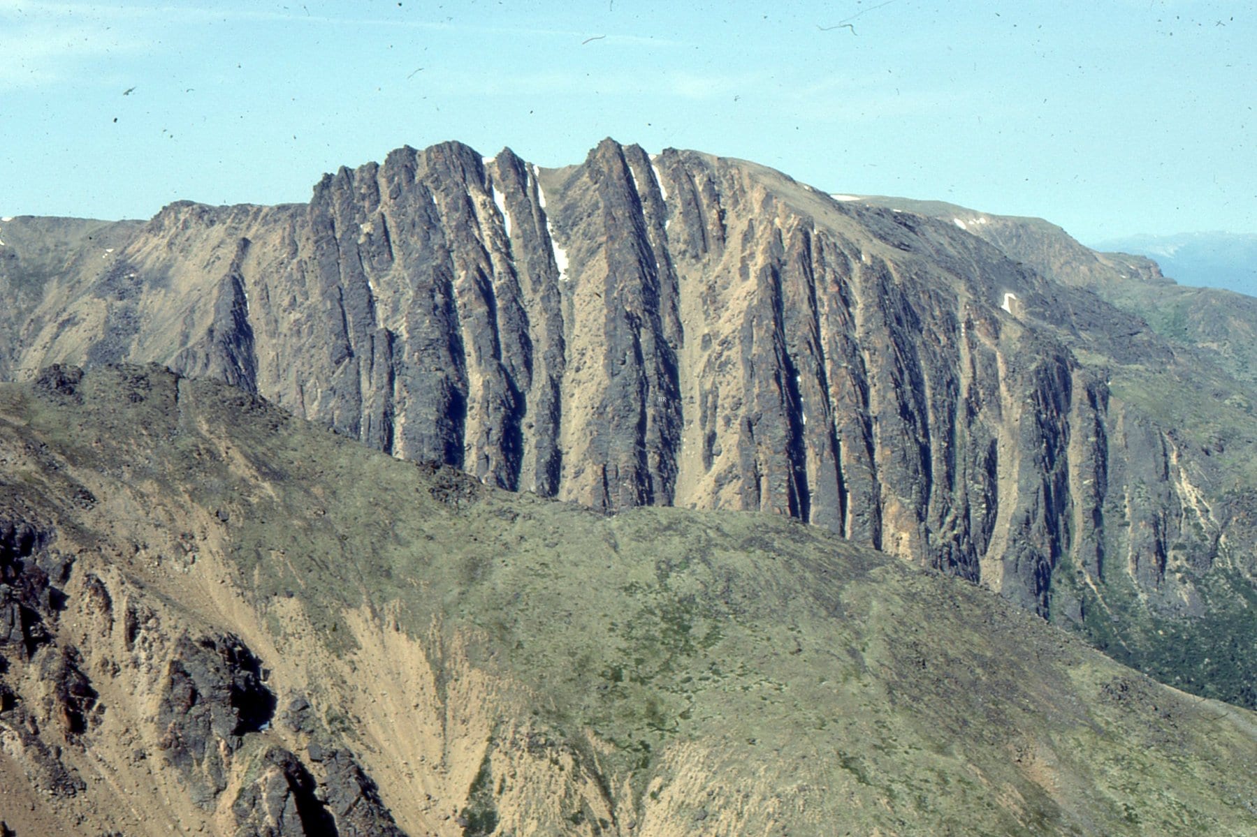
A mountain of 4th-5th order cycles that make up the larger 3rd order outer shelf to fluvial cycle. ‘X’ marks the approximate location of the cycle outcrop image above. The thickness of the 3rd order cycle here is about 1100m (yellow line). The shelf succession is separated from slope shales by a string of conglomerate-filled shelf-edge gullies.
The Jurassic cycles described above are 4th or 5th order cycles. They constitute part of a much larger stratigraphic succession, shown in the panoramic view. There are dozens of these high-order cycles over the nearly 1100m stratigraphic thickness of this Jurassic shelf. The entire section is interpreted as a 3rd-order cycle, upon which the 4th-5th order cycles were superimposed. The 3rd order cycle contains a stack of 4th-5th order cycles that at the base are each interpreted as representing the transition from outer shelf to inner shelf, and at the top (brown hues – ridge line) represent shallow marine (beach) and coarse-grained fluvial environments. Thus, the 3rd order cycle displays overall a shallowing upward trend, mimicking the much thinner 4th and 5th order cycles.
The 4th-5th order cycles correspond to parasequences in Sequence Stratigraphic terminology. Patterns of 4th-5th order cycle, or parasequence stacking, like those illustrated here, are critical elements in the recognition and interpretation of Stratigraphic Sequences – this is the topic of another post.
This is part of the How To…series on Stratigraphy and Sequence Stratigraphy
Other posts in this series on Stratigraphy and Sequence Stratigraphy
Stratigraphic surfaces in outcrop – baselevel fall
Stratigraphic surfaces in outcrop – baselevel rise
A timeline of stratigraphic principles; 15th to 18th C
A timeline of stratigraphic principles; 19th C to 1950
A timeline of stratigraphic principles; 1950-1977
Baselevel, Base-level, and Base level
Sediment accommodation and supply
Autogenic or allogenic dynamics in stratigraphy?
Sequence stratigraphic surfaces
Shorelines and shoreline trajectories
Stratigraphic trends and stacking patterns
Stratigraphic condensation – condensed sections
Depositional systems and systems tracts
Which sequence stratigraphic model is that?