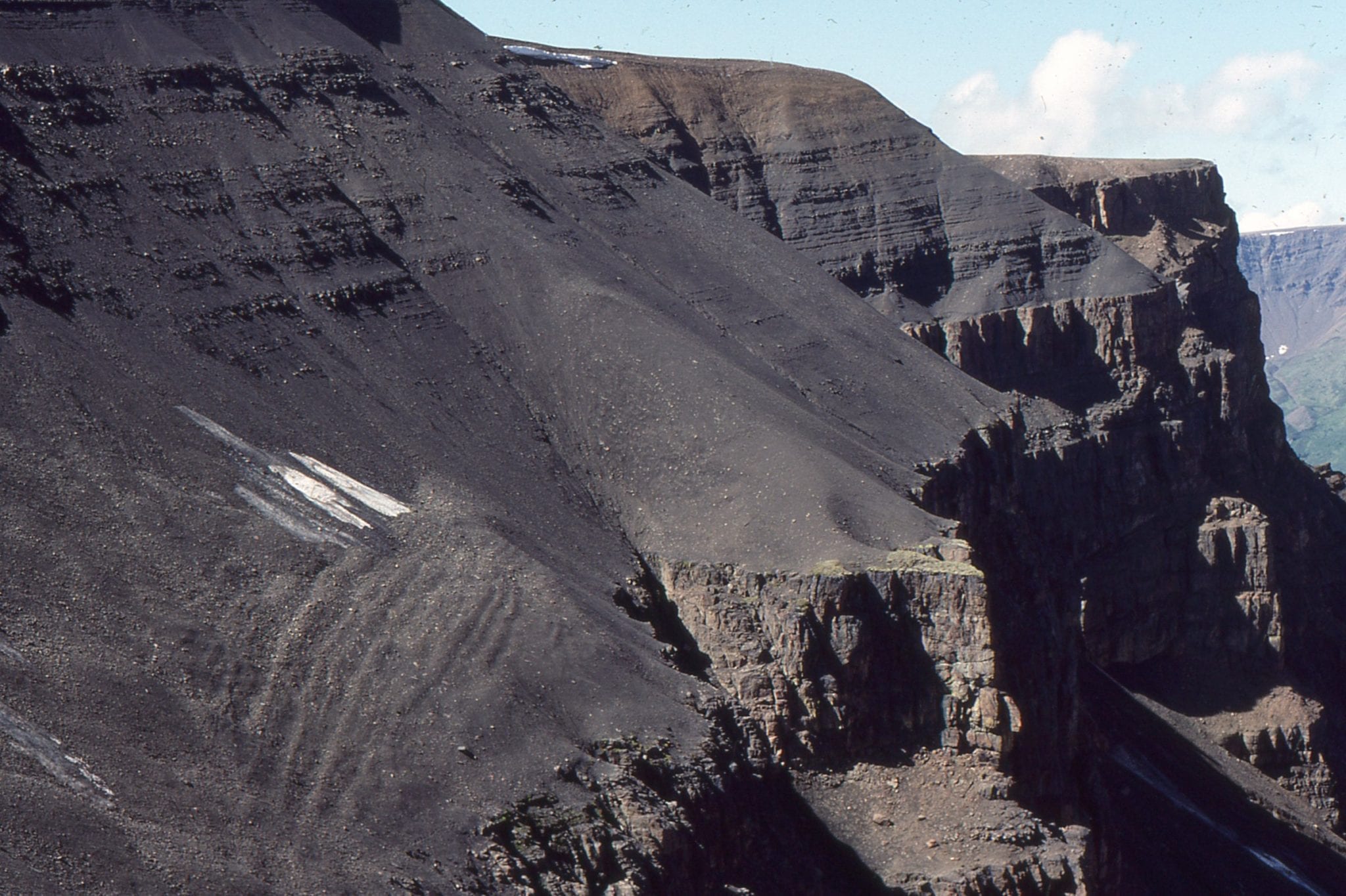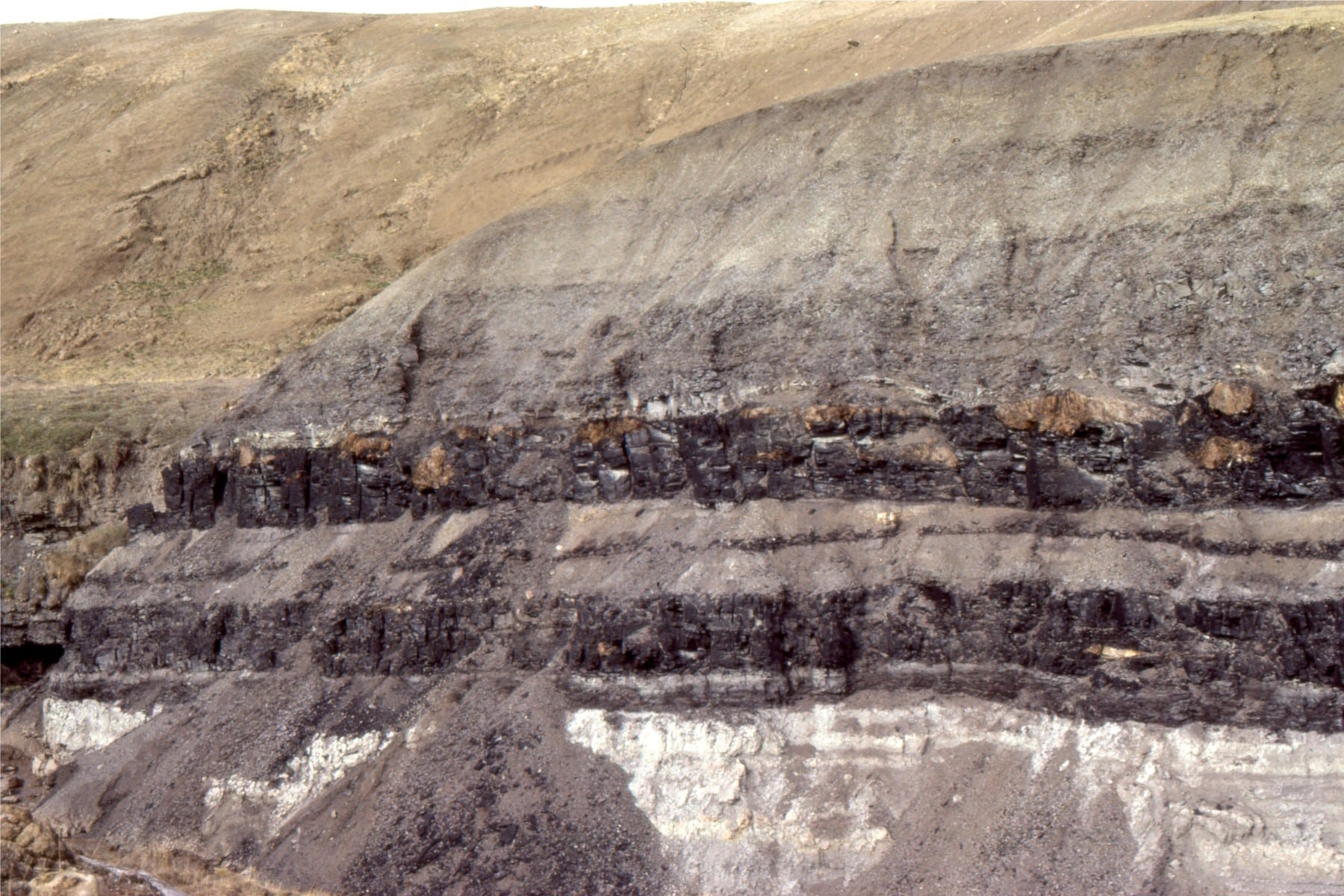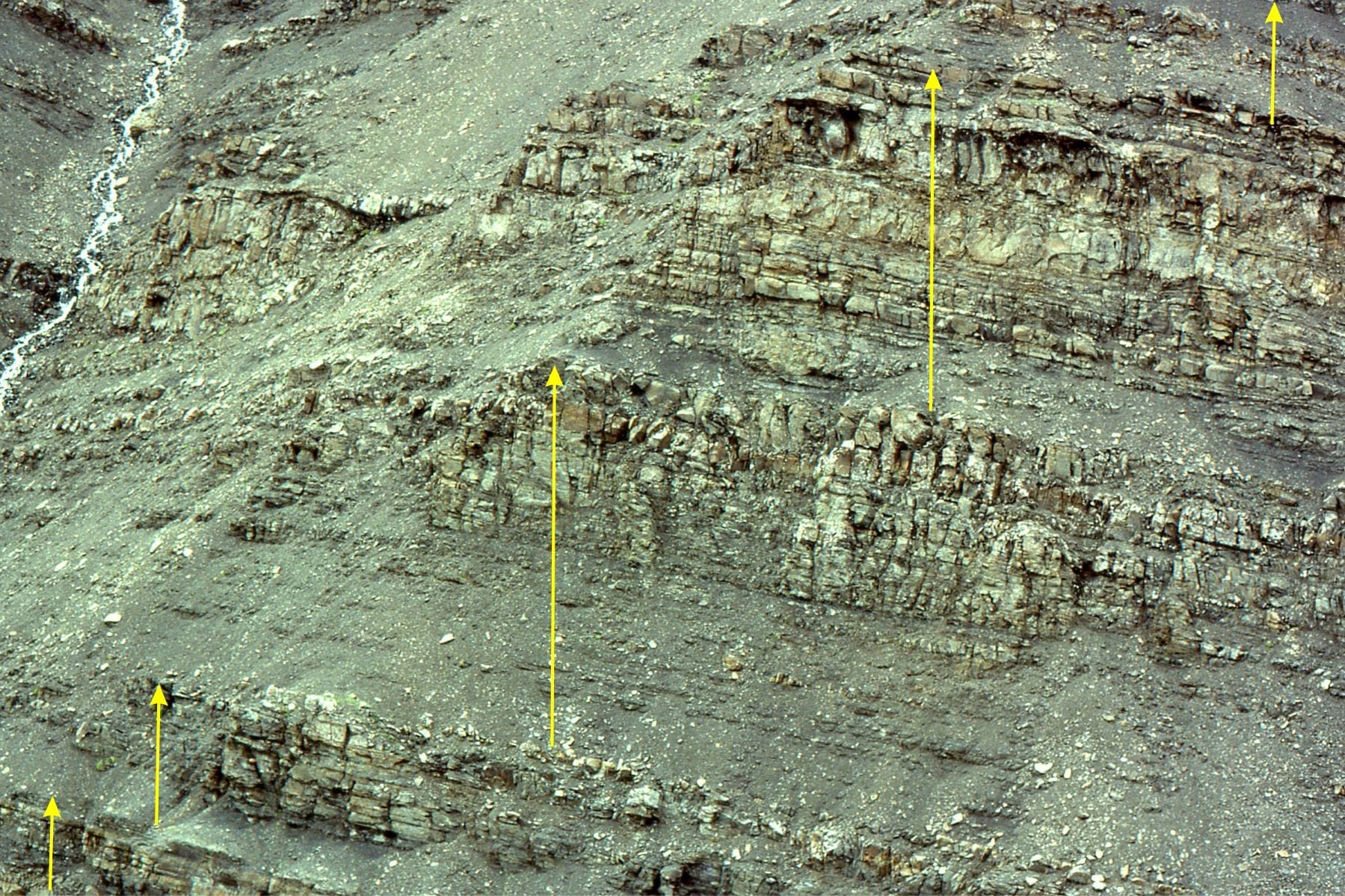
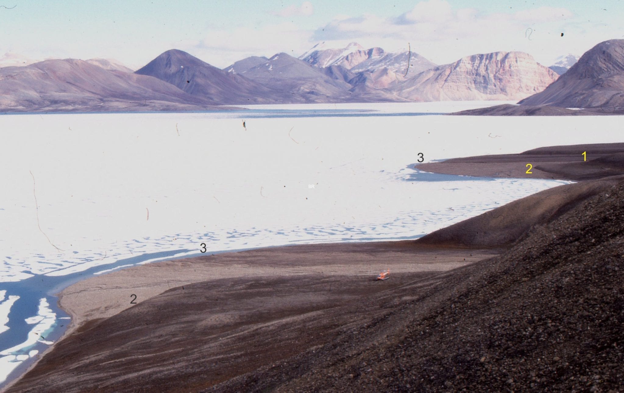
Postglacial rebound has resulted in forced regression of the shoreline along these small fan deltas. The numbers indicate approximate positions of shorelines, 1 being the oldest. Each successive shoreline and associated fan delta deposits downstep towards the modern coast. Helicopter lower right. This is Emma Fiord, Ellesmere Island in 1987.
Assessing different sequence stratigraphic models.
The concept of unconformity-bound sequences was first proposed by Sloss et al. (1949, Sloss (1963) for continent-wide Phanerozoic successions. The unconformities were formed during prolonged subaerial exposure and erosion along basin margins. However, subaerial unconformities form landward of any shoreline and, except where shallow marine and non-marine strata interfinger, the Sloss model cannot be used for coeval marine successions. All this changed in 1977 when the AAPG published Memoir 26; Seismic Stratigraphy: Applications to Hydrocarbon Exploration. Here, sequence stratigraphy was introduced as a new method of stratigraphic analysis. The method recognises that the sedimentary record is organized into discrete, but genetically related stratal packages bound by key stratigraphic surfaces, surfaces that repeat through time and are dynamically controlled by changes in baselevel: the surfaces include subaerial unconformities, maximum regressive, maximum flooding, forced regression, and ravinement surfaces, plus their correlative conformities.
The new method divided stratigraphic successions into depositional sequences, each sequence bound by subaerial unconformities and their correlative conformities. Each sequence consists of systems tracts, each systems tract contains several depositional systems, and each depositional system contains lithofacies and lithofacies associations.
The challenge to traditional lithostratigraphy (formations, members etc.) was a watershed in the science of stratigraphy and the way we think about sedimentary basins. Fundamental differences between the two methods of analysis include:
- Lithostratigraphy is deemed an objective approach to stratigraphic analysis, where interpretation plays no role in defining a formal stratigraphic unit; the starting point for sequence stratigraphy is the basic (objective) description of sedimentary rocks and sedimentary facies, but beyond this the analysis becomes more interpretive, or genetic. For example, identification of a particular depositional system relies on the interpretation of process-response characteristics of sedimentary facies.
- The fundamental lithostratigraphic units are formations which are inherently diachronous; the key stratigraphic surfaces in sequence stratigraphy have chronostratigraphic significance – the case for this was derived from the analysis of seismic reflections.
- The early proponents of sequence stratigraphy (1977 to 1988) proposed that sequences and their systems tracts were controlled primarily by eustatic changes in baselevel – hence the designation of highstand, falling stage, lowstand, transgressive, and regressive systems tracts. This proposal met with a great deal of criticism, primarily because it tended to filter out the variable effects of tectonism, basin subsidence, sediment supply, and the influence of autogenic processes on stratigraphic architecture.
Today, there is less emphasis on eustatic drivers, and more on how sequences develop during a complete cycle of changes in sediment accommodation, baselevel, and sediment supply.
[Note: In addition to AAPG Memoir 26, an excellent collection of papers in SEPM Special Publication 42 (1988) discuss important modifications and challenges to the original sequence stratigraphic model.]
The evolution of sequence stratigraphic models
Any scientific model of worth will be tested – and tested again. Models frequently undergo modification to account for any deficiencies or are replaced by new models. Sequence stratigraphy is no different; the original model (Vail and others) has gone through several iterations, including two proposals for alternative models. Most of the changes are based on different interpretations of the timing of events that produce key stratigraphic surfaces and systems tracts in relation to fluctuating baselevels, as well as the preservation potential for surfaces like the basal surface of forced regression. One problem of note is the contentious issue of identification and timing of correlative surfaces, or correlative conformities. For example, a subaerial unconformity develops during baselevel fall and the ensuing regression; this surface forms down depositional dip as the shoreline shifts basinward; the hiatus is a minimum at the youngest shoreline. At any time during this basinward shift there will be a correlative conformity in the marine parts of the basin – shelf, slope, and beyond. So, which correlative conformity does one choose – the one at the beginning of regression, the one at the end of regression, or somewhere in between? Identification of a correlative conformity in the stratigraphic record poses an additional problem; tracking seismic reflections across a basin is reasonably successful but putting one’s finger on a particular bedding plane in outcrop, core, or wireline logs is far less so, particularly in deposits that accumulate basinward of storm wave-base.
The diagram below (modified from Catuneanu et al, 2010) shows some of the important steps in this iterative process.
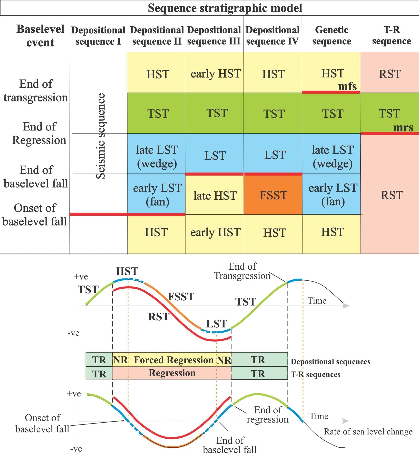
Summary of the 6 sequence stratigraphic models, their systems tracts, sequence boundaries, and the relationship between their bounding surfaces and stages of baselevel change. Modified from Catuneanu et al. 2010, Figure 2. Systems tracts abbreviations are: HST = highstand, LST = lowstand, TST = transgressive, FSST = Falling stage, and RST = regressive, mfs = maximum flooding surface, mrs = maximum regressive surface. On the sea level curve, NR = normal regression, TR = transgression
Depositional sequence I is the original model proposed by Vail, Mitchum and others in AAPG Memoir 26 (1977), based on seismic stratigraphy. The sequence boundary is a subaerial unconformity and its correlative conformity, that begin to form at the onset of baselevel fall.
Model II (e.g. Posamentier et al. 1988) maintains the sequence boundary of Model I and is divided into four systems tracts; the HST, LST, TST, and a shelf margin systems tract. There was also an attempt to clarify issues with the correlative conformity at the base of the lowstand fan. At this juncture, the Exxon group proposed two types of sequence based on the degree of erosion beneath a subaerial unconformity and its down-dip extent: Type 1 sequences are bound by a subaerial unconformity that extends to the edge of the shelf, the associated facies also transiting seawards. The subaerial unconformity bounding a Type 2 sequence is confined to the basin margin. Type 2 sequences also contain the shelf margin systems tract (SMST) which overlies the sequence boundary and is overlain by a transgressive surface. Thus, the SMST accumulates during baselevel fall. Amidst the confusion that followed, several problems quickly became apparent with this scheme (Embry, 2002; Catuneanu, 2006):
- Distinguishing between Type 1 and Type 2 unconformities was quite subjective.
- The shelf margin and lowstand systems tracts are basically the same thing; they both form from sediment shed off the basin margin and shelf during baselevel fall. One problem here is that if a Type 2 sequence was identified, then a shelf margin systems tract must follow. In other words, the model was determining whether a shelf margin or lowstand systems tract was present, rather than the nature of the rocks themselves.
- The correlative conformity basinward of the subaerial unconformity occurs within the lowstand deposits, and
- In many parts of a marine basin, the correlative conformity has “little objective expression” (quoted in Embry, 2002); in other words, there may be little or no stratigraphic and sedimentologic criteria upon which one could identify such a boundary.
Depositional model III attempts to rectify these problems by combining sequence Types 1 and 2 and moving the sequence boundary to the end of baselevel fall (i.e. the beginning of baselevel rise) (e.g. Van Wagoner et al, 1988). The shelf margin systems tract was also discarded. In this version, the former lowstand fan deposits become part of the late highstand systems tract. However, the beginning of baselevel rise does not coincide with the end of regression – regression continues for some time because there is plenty of sediment available in shallow marine environments. Thus, there may be no specific stratigraphic record of any surface that indicates the start of sea level rise.
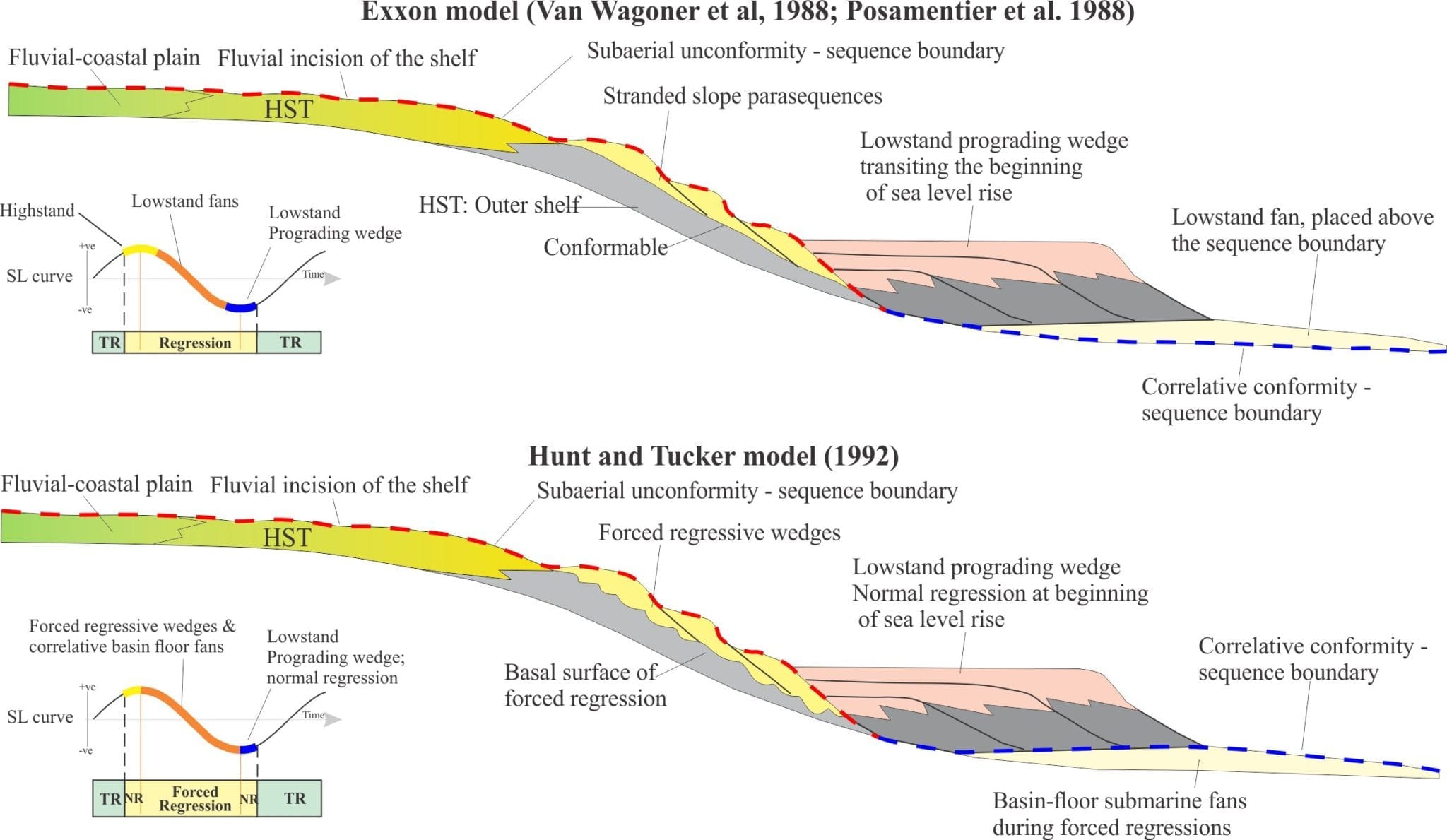
Comparison of the Exxon systematics corresponding to Model III, and the changes wrought by Hunt and Tucker (1992) in Model IV. Note the different placements of the correlative conformity (sequence boundary), the inclusion of a forced regressive systems tract that includes the down-stepping shoreface wedges and the correlative fan deposits, and the lowstand prograding wedge in the normal regressive portion of early baselevel rise. Modified from Hunt and Tucker, 1992.
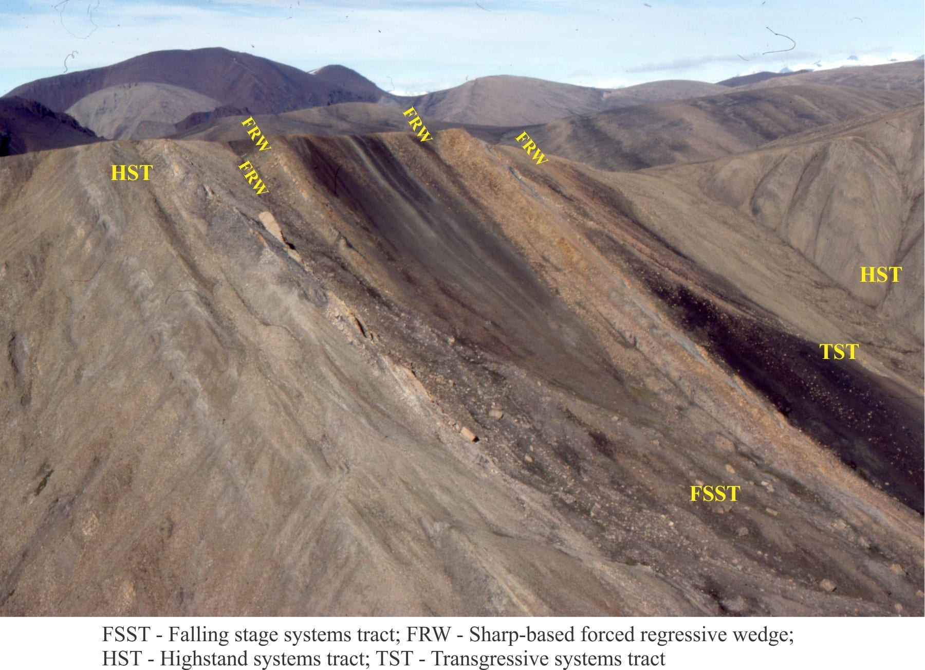
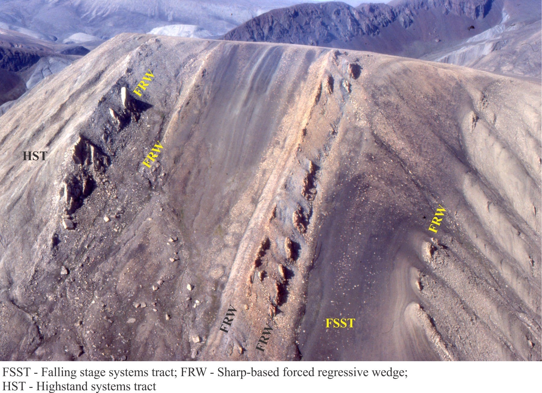
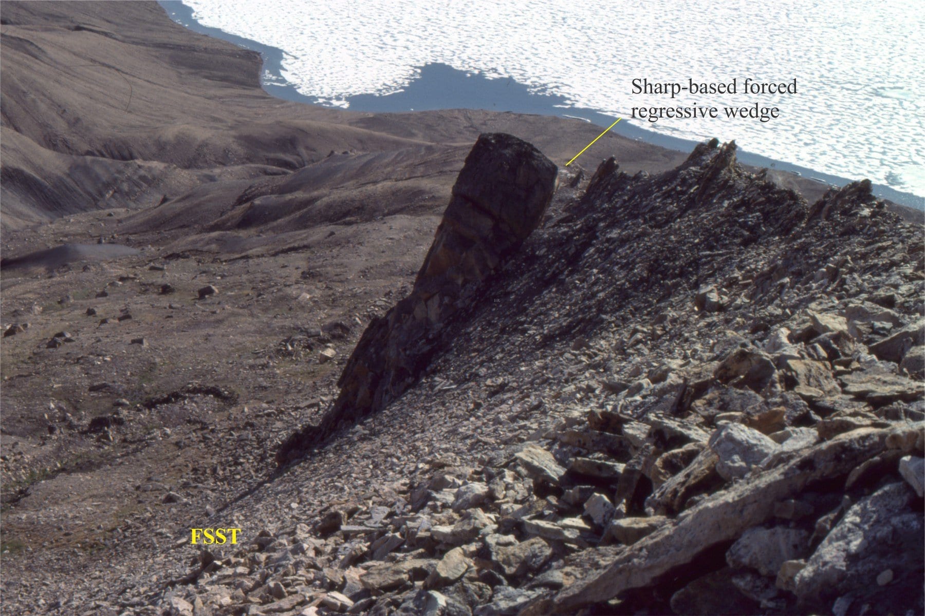
Depositional model IV is, perhaps, the first significant departure from the original Exxon story. It was based on the recognition that forced regression occurs when sediment supply is less than the rate of baselevel fall (progradation and aggradation require sediment supply to exceed baselevel fall). To account for this dynamic in the sequence stratigraphic model a falling stage systems tract (FSST) was added by Plint (1988) and Hunt and Tucker (1992). The lower boundary is the basal surface of marine erosion. A subaerial unconformity occurs at the top of the FSST, stepping downward in concert with the shoreline trajectory; the correlative conformity is placed at the base of the redefined lowstand systems tract. Here, the LST begins with the final stages of baselevel fall and continues during normal regression in the early stage of baselevel rise; it overlies the basinward part of the FSST. Of all the depositional sequence model iterations, the Hunt and Tucker scheme is the probably the most accepted.
Two alternative models:
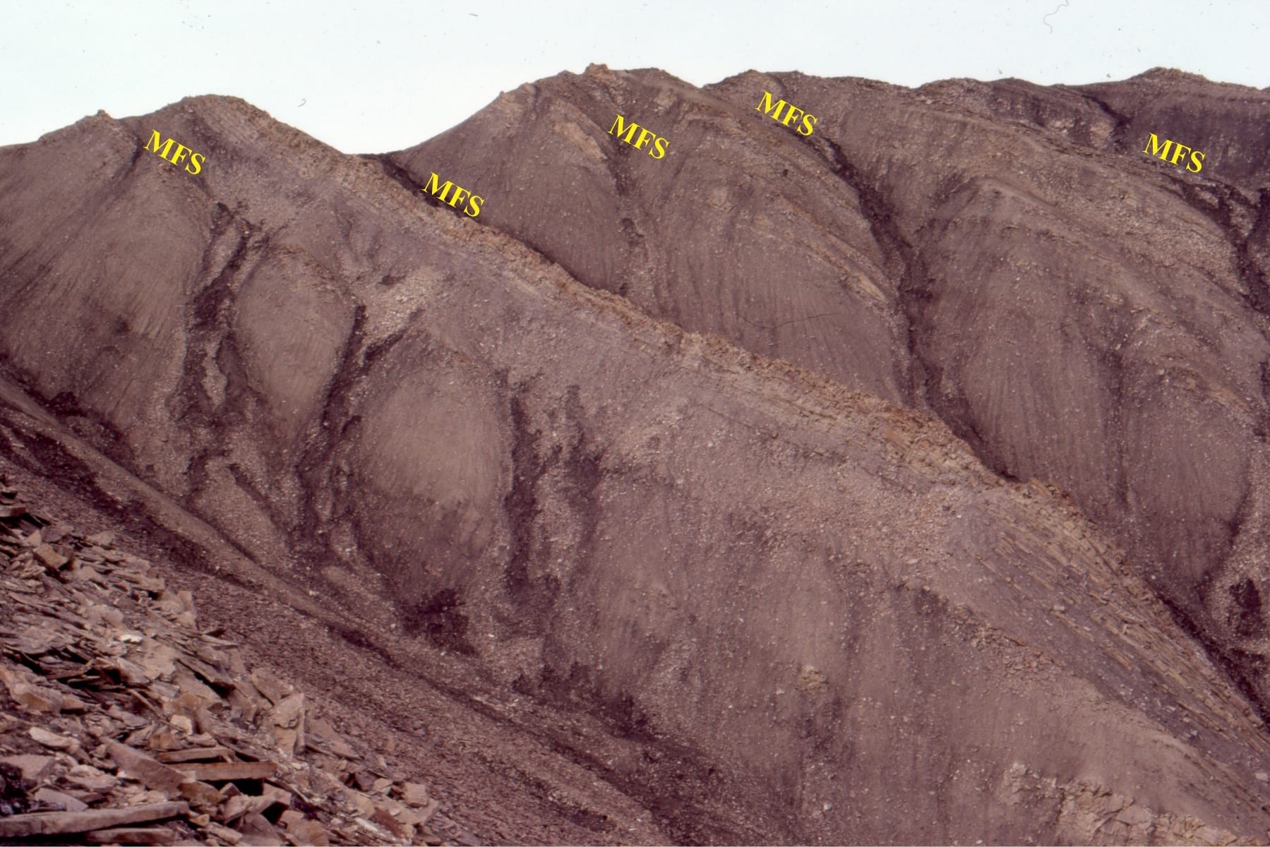
Genetic sequences (Galloway, 1989) are bound by maximum flooding surfaces (MFS). Galloway’s model relies on Frazier’s (1974) definition of depositional episodes, that represent time-bound units of progradation, aggradation and retrogradation, and form in response to transgression and regression. A Genetic sequence is the stratigraphic record of a depositional episode. Although a Genetic sequence records changes in baselevel, it is not tied to eustatic cycles – in fact, Galloway’s model was partly an attempt to extricate sequence stratigraphy from the idea that eustasy was the driving force. It was also a kind of plea for stratigraphy to return to objective lithofacies analysis, rather than being model driven.
The MFS was chosen as the Genetic sequence boundary because:
- It is the surface that signals the end of transgression and landward shoreline excursion, and the beginning of regression (note that the end of transgression does not coincide with the end of baselevel rise).
- It has low diachroneity.
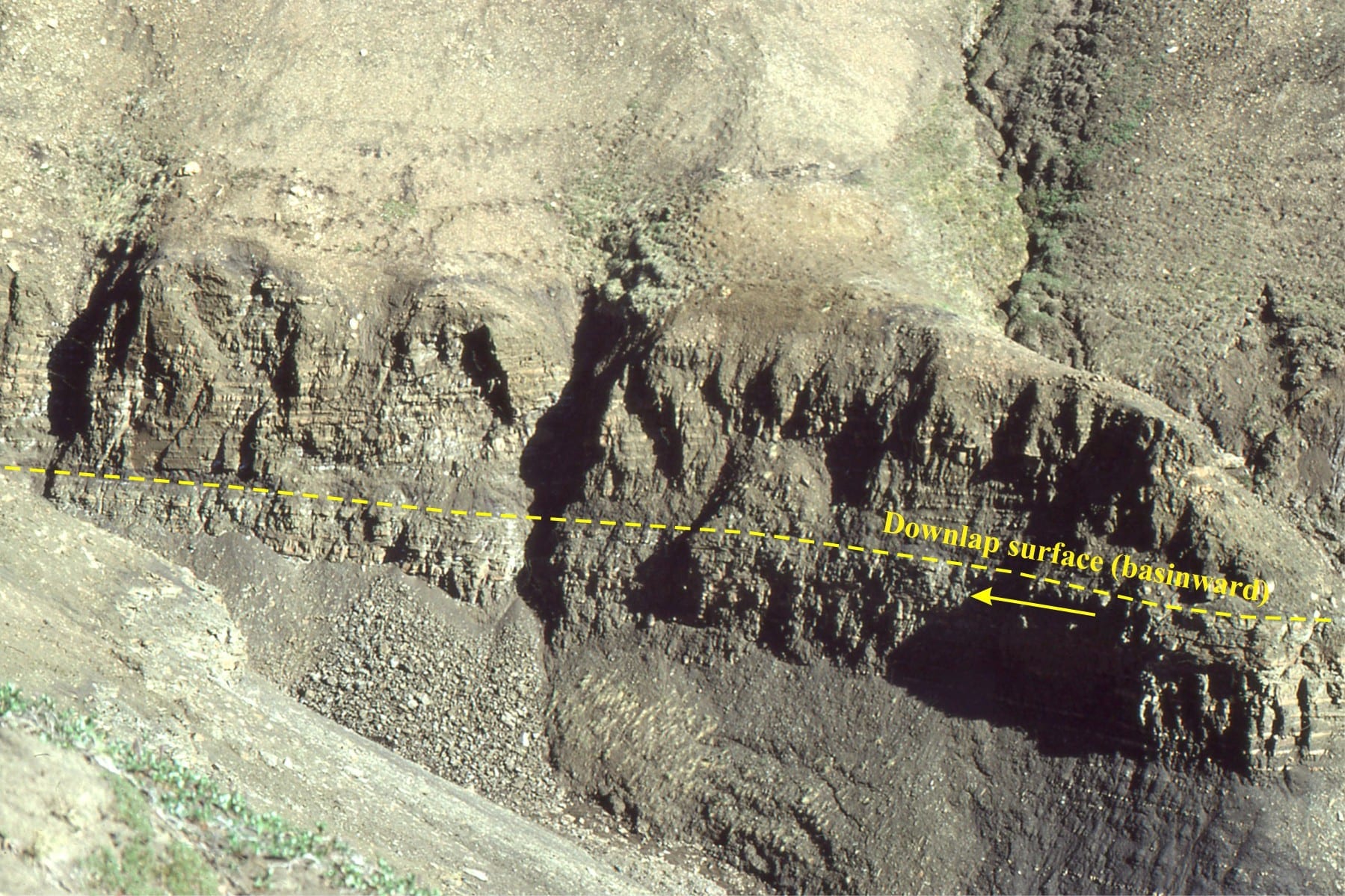
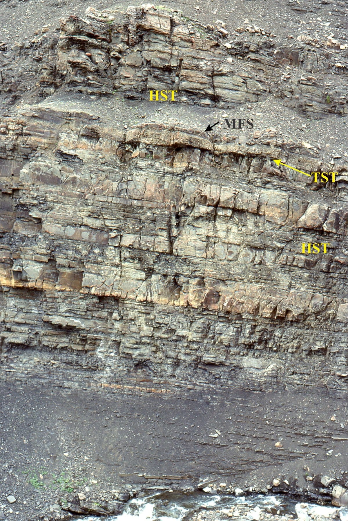
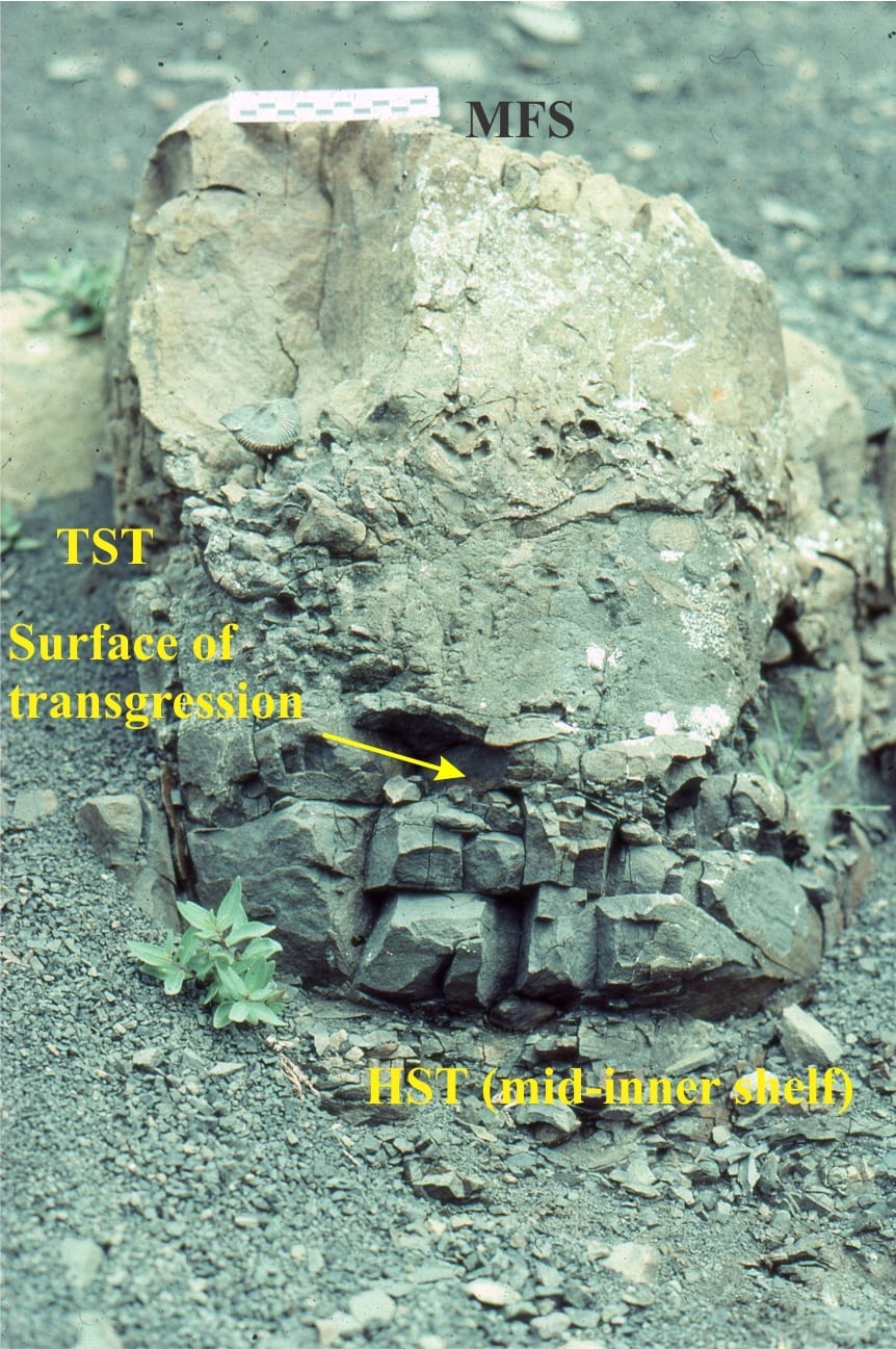
- It is an easily recognizable and mappable surface. Maximum flooding surfaces commonly overlie condensed sections or omission surfaces; they signal an abrupt lithological change from coarse-grained or cemented lithologies, to fine-grained beds that indicate the beginning of regression.
- The MFS can be traced into coeval non-marine deposits where they interfinger with marine strata; Galloway maintains that the surface can also be traced to deeper parts of the basin.
- The MFS is the only surface that can, in principle, be used across all parts of a basin.
A major criticism of Galloway’s scheme is that subaerial unconformities occur within a sequence, which means that it can no longer be considered as a relatively conformable stratigraphic unit. And unless the correlative conformity coincides with a condensed section or omission surface, its identification in deep water strata suffers from the same kinds of problems that the other models contend with.
Transgressive-regressive (T-R) sequences
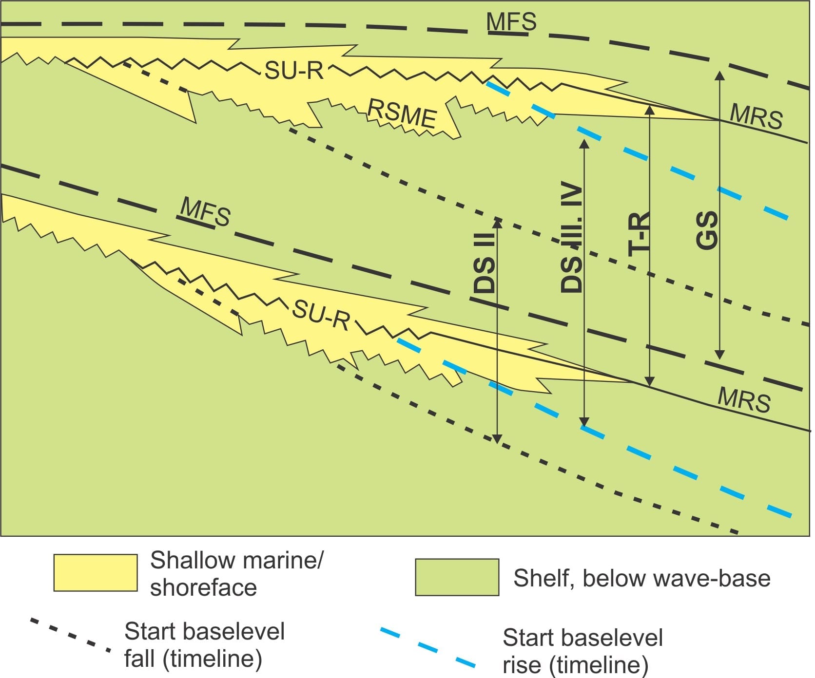
Sequence stratigraphic models according to Embry (2002), including Genetic sequences (GS) and T-R sequences. The boundaries of depositional sequence (DS) models II and III are also indicated. SU-R = subaerial unconformity – ravinement surface, RSME = regressive surface of marine erosion at the base of each forced regressive wedge.
The general plan of attack for T-R sequences was formulated by Embry and Johannessen (1993). T-R sequences are bound by subaerial unconformities and their marine equivalents, maximum regressive surfaces (MRS); the subaerial unconformity may be partly or wholly replaced by a ravinement surface. This model avoids the complications of correlative conformities in shallow marine strata and maintains the general mantra of relatively conformable successions (unlike Genetic Sequences). The relative ease of identification of the bounding surfaces in outcrop and seismic profiles gives this model some advantage over its predecessors. T-R sequences contain only regressive and transgressive systems tracts; the boundary at the top of the TST is the maximum flooding surface.
However, like depositional sequences, there is a common problem of identifying the correlative conformity in deep water deposits including the deep shelf seaward of storm wave-base, and slope-submarine fan deposits that are dominated by sediment gravity flows and mass transport deposits (slumps, slides etc.). An additional problem is the claim that the MRS has low diachroneity which, as Catuneanu (2006) and others have noted, may be true along depositional dip, but not along depositional strike because of significant variations in sedimentation rates from one part of the basin margin to another.
The regressive component of T-R sequences assembles the highstand, falling stage, and lowstand systems tracts of depositional and Genetic sequences into a single stratigraphic entity (RSTs). This has the advantage of simplicity. But there is also an advantage in knowing which components derived from normal and forced regression – this information helps us understand basin dynamics. This can still be done by identifying the relevant depositional systems within the RST, but there is no explicit inclusion of the corresponding systems tracts within the T-R model.
Which model is best?
If the geological literature is anything to go by, one might assume that the Exxon-type depositional sequence schemas are the only models worth considering; Genetic and T-R sequence models barely get a mention. And yet there are as many advantages and disadvantages to depositional sequence schemes as there are for the two alternatives. Perhaps it’s a function of shouting loudest. To compound the issue, it is not always clear in many publications which depositional sequence version is being used.
A group of stratigraphers has grappled with these problems, publishing their deliberations and recommendations in several papers (e.g. Catuneanu et al. 2010, and 2011). The group acknowledges the historical significance of the depositional sequence models introduced by Vail and his colleagues, but not their primacy. Several conclusions stand out:
- All the models have value, they are all sensible and logical; each has advantages and disadvantages.
- No single model solves all stratigraphic problems.
- The fundamental basis for stratigraphic interpretation is sound lithofacies analysis.
- Choose the model that best suits the geological environment and the available data: interpretation of the stratigraphy should be based on geology and not driven by a model.
- Identify this model in your reporting.
This is sound advice!
This post is part of the How To…series on Stratigraphy and Sequence Stratigraphy
Other posts in this series on Stratigraphy and Sequence Stratigraphy
Stratigraphic surfaces in outcrop – baselevel fall
Stratigraphic surfaces in outcrop – baselevel rise
A timeline of stratigraphic principles; 15th to 18th C
A timeline of stratigraphic principles; 19th C to 1950
A timeline of stratigraphic principles; 1950-1977
Baselevel, Base-level, and Base level
Sediment accommodation and supply
Autogenic or allogenic dynamics in stratigraphy?
Stratigraphic cycles: What are they?
Sequence stratigraphic surfaces
Shorelines and shoreline trajectories
Stratigraphic trends and stacking patterns
Stratigraphic condensation – condensed sections
Depositional systems and systems tracts